Solving ODEs Numerically

When you cannot solve it by hand

The differential-equations lesson showed how to solve linear ODEs analytically. Most real engineering models — nonlinear, coupled, driven by messy inputs — have no closed-form solution, so we solve them numerically: start from a known initial condition and step the solution forward in small increments. The problem is the initial value problem,

and a numerical method approximates \(y\) at a sequence of times \(t_0, t_1, \dots\) spaced by a step size \(h\) ¹.

Euler’s method

The simplest scheme follows the slope the equation gives. At each step, use the derivative at the current point to extrapolate forward:

This is Euler’s method. It is intuitive — “take a small step in the direction the equation points” — but only first-order accurate: halving the step roughly halves the error, so an accurate solution needs many tiny steps. With a coarse step the approximation visibly drifts away from the truth, as the dashed curve in the figure shows for \(\frac{dy}{dt} = -y\) (whose exact solution is \(e^{-t}\)).

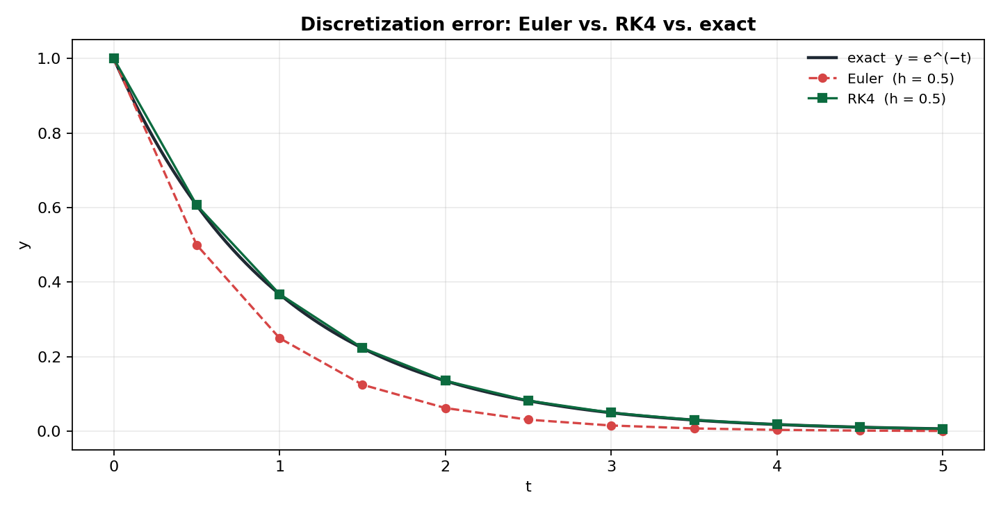
Better steps: Runge–Kutta

Most production solvers do something smarter than a single slope sample. The classic fourth-order Runge–Kutta (RK4) method samples the slope four times across each step and combines them in a weighted average, achieving fourth-order accuracy — error shrinks like \(h^4\) ¹. At the same coarse step where Euler drifts, RK4 (solid green) sits almost on top of the exact curve. That accuracy-per-step is why higher-order methods dominate in practice.

There is always a trade-off: smaller steps and higher order mean more accuracy but more computation, and some “stiff” problems demand special implicit methods to stay stable. Choosing the method and step size is part of the engineering.

In practice: use a tested solver

You rarely hand-code these. SciPy provides robust, adaptive solvers that choose their own step sizes to meet an error tolerance ²:

import numpy as np
from scipy.integrate import solve_ivp

def f(t, y):
    return -y                      # dy/dt = -y

sol = solve_ivp(f, t_span=(0, 5), y0=[1.0],
                t_eval=np.linspace(0, 5, 100))
# sol.t, sol.y hold the solution to compare against exp(-t)

solve_ivp defaults to an adaptive Runge–Kutta method and handles step-size control for you. The lesson of the figure still applies, though: numerical solutions are approximations, and understanding error and stability is what keeps you from trusting a plot that has quietly drifted from reality.