Linear Systems and Gaussian Elimination

A system of equations is a matrix equation

A system of linear equations is a collection of equations in which each unknown appears only to the first power, with no products of unknowns. For example,

Each equation contributes one row of coefficients. Collecting those coefficients into a matrix \(A\), the unknowns into a vector \(\mathbf x\), and the right-hand sides into a vector \(\mathbf b\), the whole system becomes the single matrix equation \(A\mathbf x=\mathbf b\):

Reading the matrix-vector product row by row reproduces the three equations exactly. Solving the system means finding every \(\mathbf x\) for which \(A\mathbf x=\mathbf b\) holds ¹.

The augmented matrix and elementary row operations

Because the unknowns just label columns, we can drop them and track only the numbers. The augmented matrix \([A\mid\mathbf b]\) places \(\mathbf b\) as an extra column to the right of \(A\):

Gaussian elimination transforms this matrix using three elementary row operations, each of which leaves the solution set unchanged: (1) swap two rows; (2) multiply a row by a nonzero constant; (3) add a multiple of one row to another. The goal is row echelon form, in which each row’s leading nonzero entry (its pivot) sits to the right of the pivot above it, producing a staircase of zeros in the lower-left ¹.

A worked 3x3 example

Use row 1 to clear the first column. Add \(\tfrac{3}{2}\) times row 1 to row 2, and add row 1 to row 3:

Now clear the second column below the new pivot \(\tfrac12\). Subtract \(4\) times row 2 from row 3 (since \(2/\tfrac12=4\)):

This is row echelon form, with pivots in all three columns. Now apply back-substitution, working from the bottom up. The last row says \(-x_3=1\), so \(x_3=-1\). The middle row says \(\tfrac12 x_2+\tfrac12 x_3=1\); substituting \(x_3=-1\) gives \(\tfrac12 x_2-\tfrac12=1\), so \(x_2=3\). The top row says \(2x_1+x_2-x_3=8\); substituting gives \(2x_1+3+1=8\), so \(x_1=2\). The solution is

You can verify it satisfies all three original equations.

Reduced row echelon form

Gauss-Jordan elimination goes one step further: scale every pivot to \(1\) and clear the entries above each pivot as well as below. The result is reduced row echelon form (RREF), where each pivot column is all zeros except for its single \(1\). For our example, RREF of \([A\mid\mathbf b]\) is

which reads off the answer directly without back-substitution ¹.

Three possibilities, revealed by the pivots

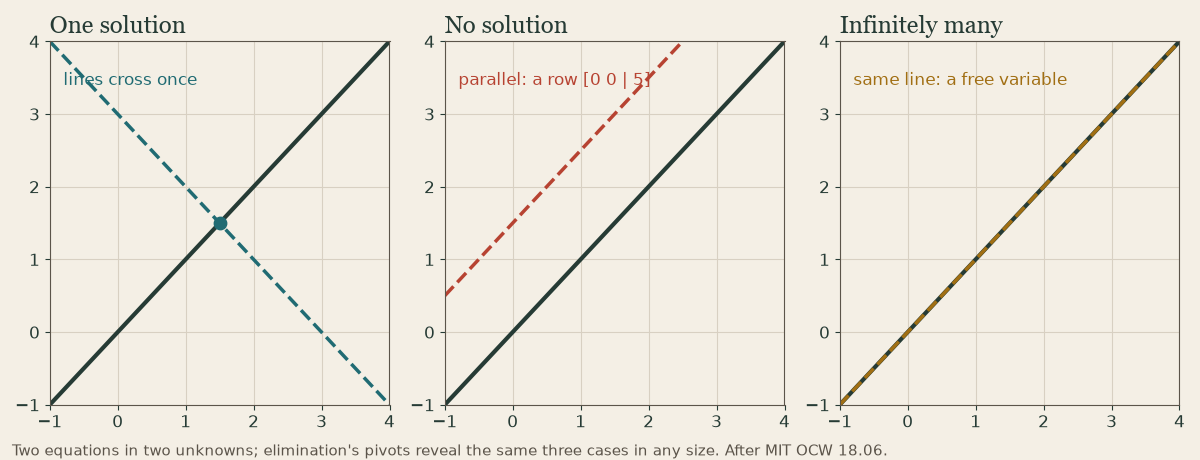
Every linear system has exactly one of three outcomes, and the echelon form tells you which. A pivot is a leading nonzero entry; a column without a pivot corresponds to a free variable that may take any value.

• Unique solution: every unknown’s column has a pivot and no contradiction appears, as in the example above.
• No solution: elimination produces a row of the form \([\,0\;\cdots\;0\mid c\,]\) with \(c\neq0\), which states \(0=c\) — an impossibility. The system is inconsistent.
• Infinitely many solutions: the system is consistent but at least one column lacks a pivot. Each free variable can be chosen freely, and the pivot variables are then determined in terms of them ¹.

The rank of \(A\) is the number of pivots — equivalently, the number of independent equations. For an \(n\)-unknown system, a unique solution requires rank \(n\); a smaller rank leaves \(n-\text{rank}\) free variables.

The inverse, and why elimination is preferred

When \(A\) is square and has full rank (a pivot in every row and column), it is invertible: there is a matrix \(A^{-1}\) with \(A^{-1}A=I\). Multiplying \(A\mathbf x=\mathbf b\) on the left by \(A^{-1}\) gives the closed form

This is conceptually clean, but in practice you rarely compute \(A^{-1}\). Forming the inverse takes more arithmetic than elimination, amplifies rounding error, and discards the structure that makes elimination efficient. The standard advice is to solve \(A\mathbf x=\mathbf b\) directly by elimination rather than building and applying an inverse ¹.

Why engineers care

Linear systems are everywhere in engineering analysis. In circuits, nodal analysis writes Kirchhoff’s current law at each node, yielding a system whose unknowns are the node voltages. In statics, the equilibrium equations that force and moment sum to zero produce linear systems for unknown reaction forces in trusses and frames. And throughout numerical methods — finite-element and finite-difference solvers, regression, optimization — the core computational step is solving a large \(A\mathbf x=\mathbf b\). Mastering elimination, pivots, and rank gives you both the hand technique for small systems and the conceptual map for the algorithms that handle the large ones.