Kinematics in One and Two Dimensions

Describing motion

Kinematics describes how things move without yet asking why — that “why” is the next lesson on forces. Motion is built from three quantities, each the calculus rate of the one before it ¹. Position \(x(t)\) locates the object; velocity is its rate of change,

and acceleration is the rate of change of velocity, \(a = \dfrac{dv}{dt} = \dfrac{d^2x}{dt^2}\). These are the same derivatives from the math course, now attached to physical meaning: velocity is the slope of the position graph, acceleration the slope of the velocity graph.

Constant-acceleration equations

A great many problems involve (at least approximately) constant acceleration — most famously free fall near Earth’s surface, where \(a = -g\) with \(g \approx 9.8\ \text{m/s}^2\). Integrating \(a = \text{const}\) twice gives the three kinematic equations that solve nearly every introductory motion problem ¹:

The third is the time-free combination — useful when you know distances and speeds but not the elapsed time. Choosing which equation to use is mostly a matter of identifying which quantity is missing.

Two dimensions: independent components

Motion in a plane is not a new theory — it is two one-dimensional problems running at once. The key insight is that the horizontal and vertical components are independent: gravity affects the vertical motion and leaves the horizontal motion untouched ¹. A velocity at angle \(\theta\) splits into \(v_x = v\cos\theta\) and \(v_y = v\sin\theta\), and each component obeys the one-dimensional equations above on its own.

Projectile motion

The classic application is the projectile: launched at speed \(v_0\) and angle \(\theta\), with gravity the only force. Horizontally the motion is uniform (\(a_x = 0\), so \(x = v_0\cos\theta\, t\)); vertically it is uniformly accelerated (\(a_y = -g\)). Eliminating time gives the parabolic path shown below.

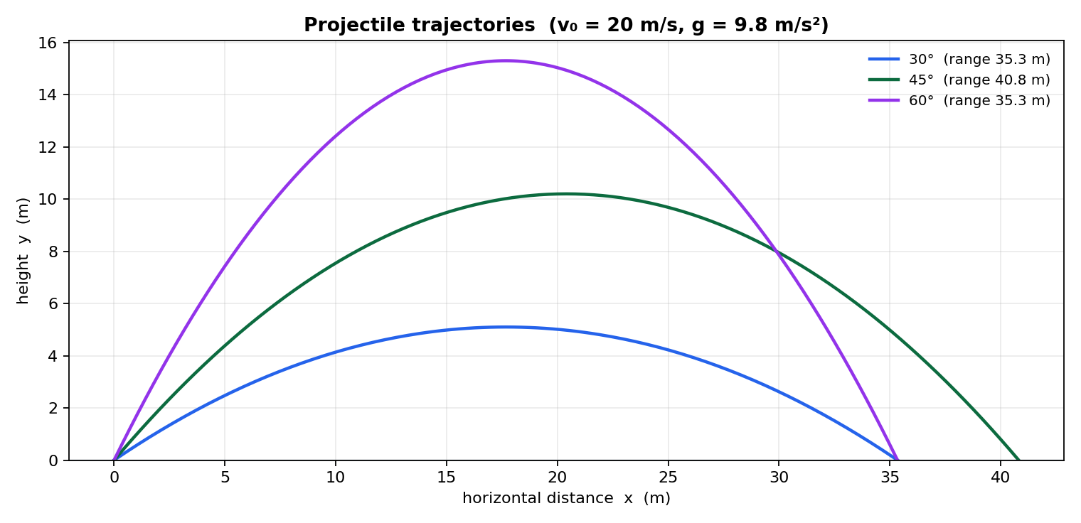
From the components you can derive the familiar results — the time of flight, the peak height, and the range on level ground,

which is maximized at \(\theta = 45^\circ\), as the equal-range pairing of the \(30^\circ\) and \(60^\circ\) curves in the figure hints ¹. With motion described, the next lesson introduces the forces that cause acceleration.

Stopping distance

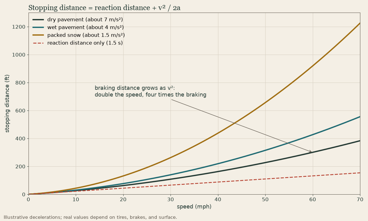
The kinematic equations are how a driver’s stopping distance is worked out. It has two parts:

• Reaction distance: during the reaction time \(t_r\) the vehicle keeps its speed, covering \(v\,t_r\).
• Braking distance: set \(v = 0\) in the time-free equation and solve: \(d = \dfrac{v^2}{2a}\).

At 60 mph (26.8 m/s) with a 1.5 s reaction, the reaction distance is 40 m. Braking at about 7 m/s² on dry pavement adds 51 m, for roughly 92 m (300 ft) in all. On packed snow, where deceleration may be nearer 1.5 m/s², braking alone takes about 240 m. Because braking distance goes as \(v^2\), doubling the speed quadruples it.

Free fall, the other everyday case: drop a stone down a well and count 2.0 s to the splash. Ignoring the sound’s travel time, \(x = \tfrac12 g t^2 = \tfrac12(9.8)(2.0)^2 \approx 20\) m.