Numerical Integration and Differentiation

From calculus to the computer

Calculus gives clean rules for derivatives and definite integrals, but those rules need a formula to differentiate or integrate. On a computer you often have something less tidy: a function you can only evaluate at points, or a set of measured samples with no formula at all. Numerical methods recover the derivative and the integral from those evaluations alone. The price is that every result is an approximation, and the central skill is understanding how large that approximation error is.

Numerical differentiation with finite differences

The derivative is a limit of slopes, so the simplest estimate just stops taking the limit and uses a small but finite step \(h\). The forward difference is

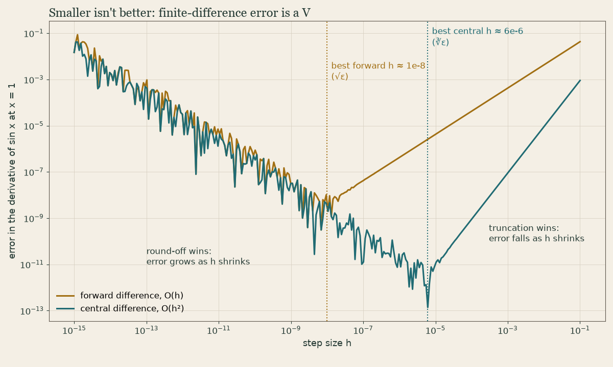
A Taylor expansion shows its error shrinks in proportion to \(h\): it is first-order accurate, written \(O(h)\). Halving \(h\) only halves the error, which is slow. A smarter choice samples symmetrically on both sides — the central difference:

Here the first-order terms cancel, leaving error proportional to \(h^2\): halving \(h\) cuts the error by four. For the same effort, the central difference is far more accurate, so prefer it whenever you can evaluate \(f\) on both sides.

It is tempting to drive \(h\) toward zero, but that fails. As shown in the floating-point lesson, subtracting two nearly equal numbers like \(f(x+h)\) and \(f(x-h)\) loses significant digits to round-off error, and dividing by a tiny \(h\) amplifies it. So two errors pull in opposite directions: truncation error falls as \(h\) shrinks, while round-off error grows. Their sum is minimized at an intermediate optimal \(h\) — for central differences, typically near the cube root of machine epsilon (roughly \(10^{-5}\) in double precision), not the smallest \(h\) you can represent.

For sampled data, NumPy’s numpy.gradient applies central differences in the interior and one-sided differences at the endpoints, returning a derivative array the same length as the input:

import numpy as np

x = np.linspace(0, np.pi, 100)
y = np.sin(x)
dydx = np.gradient(y, x)   # approximates cos(x)

Numerical integration (quadrature)

Estimating a definite integral from samples is called quadrature. The idea is to replace the curve with shapes whose area is easy to compute. Split \([a, b]\) into \(n\) equal panels of width \(h\), with sample values \(f_0, f_1, \dots, f_n\).

The trapezoidal rule connects neighboring samples with straight lines and sums the trapezoids:

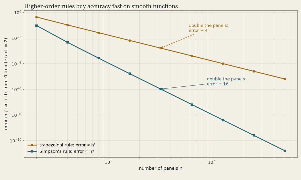
Its error is \(O(h^2)\), and it is the safe default — robust, and it makes no assumption beyond having the samples. Simpson’s rule does better by fitting a parabola through each pair of panels instead of a line. That extra curvature captures smooth functions far more accurately, with error \(O(h^4)\), so on a smooth integrand it reaches a given accuracy with many fewer points. (Simpson’s rule needs an even number of panels.) Use Simpson’s rule when the function is smooth and you want accuracy; fall back to the trapezoidal rule for noisy data or when smoothness is not guaranteed.

Why does adding up little areas recover the integral at all? The Fundamental Theorem of Calculus says the definite integral is the net signed area under the curve ¹, and that area is exactly what these rules approximate.

SciPy’s scipy.integrate module covers both situations ². When you have a callable function and want a single accurate number, quad performs adaptive quadrature, placing evaluations where the function is most curved and returning both the estimate and an error bound. When you only have sampled data, use trapezoid or simpson, which apply the rules above to your arrays:

import numpy as np
from scipy.integrate import quad, trapezoid, simpson

# A function we can evaluate anywhere: integral of sin from 0 to pi is 2.
value, err = quad(np.sin, 0, np.pi)     # value ~ 2.0, err is a bound

# The same integral from fixed samples (no formula needed downstream):
x = np.linspace(0, np.pi, 101)
y = np.sin(x)
approx_trap = trapezoid(y, x)           # ~ 1.9998
approx_simp = simpson(y, x)             # ~ 2.0000, more accurate

For the smooth sine curve, Simpson’s result lands closer to the exact value of 2 than the trapezoidal one at the same sample count — the higher-order rule earning its keep.

Choosing a method

Reach for quad when you can evaluate the function and want one trustworthy number with an error estimate. Use trapezoid or simpson when your data arrives as samples — for example, sensor readings or the output of another computation. For derivatives, prefer central differences and numpy.gradient, and resist shrinking \(h\) past the point where round-off takes over. In every case the discipline is the same: pick the rule that matches your data, then keep an eye on the error you are willing to accept.