Throughput, Bottlenecks, Buffers & OEE
How many brackets the drill cell really makes: cycle time versus takt time, finding the bottleneck, why a faster robot changes nothing if the drill is the constraint, sizing a buffer from how long the next machine stops, Little's Law (work in process = throughput × time in system), and OEE worked through Vorne's example (88.8% × 86.1% × 97.8% = 74.8%) and then for the cell.
- 5 min
- 7 steps
- 3 questions
- Lesson 65 of 78
In this lesson
- Cycle time and takt time
- Find the bottleneck
- Blocking and starving
- Buffers
- Little’s Law
- OEE
- Try it
Picking up where you left off.
Cycle time and takt time
Two numbers start every throughput conversation:
- Cycle time: how long a station takes per part.
- Takt time: how often a part must come off the line to meet demand: available time divided by required quantity.
Say the customer needs 1,000 brackets per shift, and a shift has 480 minutes minus 60 minutes of breaks, or 420 minutes (25,200 seconds) available. Takt time is 25,200 ÷ 1,000 = 25.2 seconds. Every station has to finish a part in less than 25.2 seconds on average, including its downtime.
Find the bottleneck
The cell’s three steps:
| Step | Cycle time | Parts per hour, if never stopped |
|---|---|---|
| Infeed conveyor | 5 s | 720 |
| Clamp and drill | 20 s | 180 |
| Robot unload | 12 s | 300 |
The drill is the bottleneck. The cell can’t make more than 180 an hour, and buying a faster robot or speeding up the conveyor won’t change that by one part; it only makes those machines wait longer. Improvements go to the constraint first: a faster feed rate, a second spindle, or moving the clamp time off the drill’s clock by clamping in a second fixture while the first one drills. Once the drill gets faster than 12 seconds, the robot becomes the bottleneck, and the work moves there.
MIT’s manufacturing systems course builds this whole subject, from capacity and queues to buffers and scheduling, on these ideas 1.
Quick check
The slowest step sets the pace; improve it first.
Blocking and starving
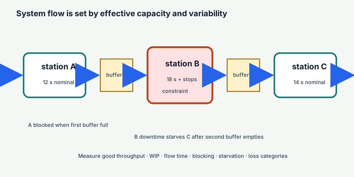
Machines in a line interact. If the robot faults, the drill finishes its part and then has nowhere to put it: it’s blocked. If the infeed jams, the drill runs out of parts: it’s starved. Either way, the bottleneck loses time, and time lost at the bottleneck is lost for the whole cell.
Buffers
A buffer is space for parts between machines, so one machine’s short stoppage doesn’t stop the next. Size it from how long stoppages actually last:
- If the robot’s typical fault takes 2 minutes to clear, the drill can keep running through it if the outfeed has room for 120 s ÷ 20 s = 6 parts.
- If the infeed jams for up to a minute, 3 parts queued ahead of the drill keep it fed.
Buffers aren’t free: floor space, parts sitting in process, and more to track. Size them from the stoppage data, not a round number, and put them on either side of the bottleneck where they protect it.
Quick check
Size buffers from how long the downstream machine actually stops.
Little’s Law
For a stable line, the average amount of work in process equals throughput times the average time a part spends in the system:
WIP = throughput × flow time
If the cell makes 150 good brackets an hour and there are, on average, 10 brackets somewhere between the infeed and the outfeed, each bracket spends 10 ÷ 150 = 0.067 hour, about 4 minutes, in the cell. Bigger buffers raise WIP; if throughput doesn’t rise with them, they just make each part wait longer. The law is one of the backbones of the MIT course 1.
OEE
Overall equipment effectiveness splits lost production into three kinds 2:
- Availability = run time ÷ planned production time (losses: breakdowns, changeovers).
- Performance = (ideal cycle time × total count) ÷ run time (losses: slow cycles, small stops).
- Quality = good count ÷ total count (losses: scrap, rework).
- OEE = availability × performance × quality.
Vorne’s worked example 2: a 480-minute shift with 60 minutes of breaks gives 420 planned minutes; 47 minutes of downtime leaves 373 minutes of run time, so availability is 88.81%. With a 1-second ideal cycle and 19,271 parts made, performance is 19,271 s ÷ 22,380 s = 86.11%. With 423 rejects, quality is 18,848 ÷ 19,271 = 97.80%. OEE is 0.8881 × 0.8611 × 0.9780 = 74.79%. World-class OEE is often quoted as 85% 2.
For the drill cell: in 420 planned minutes, the drill is down 30 minutes (availability 92.9%); in 390 minutes of running it makes 1,080 brackets against an ideal of 1,170 at 20 seconds (performance 92.3%); 22 are scrap (quality 98.0%). OEE is 0.929 × 0.923 × 0.980 = 84.0%, and good output is 1,058: enough for the 1,000-bracket demand, with not much margin.
Use the three numbers to find where the time goes, not as a score. A plant that grades people on OEE soon finds downtime getting recorded as “planned.”
Playback is optional. If the player is unavailable, open the video at its source.
Quick check
OEE multiplies the three; each loss stacks on the others.
Try it
Your demand rises to 1,200 brackets a shift. Work out the new takt time, whether the drill can meet it at 84% OEE, and what you’d change first. Then size the buffer between drill and robot if the robot’s faults last up to 3 minutes.
Lesson complete
Nice work.
Sources for this lesson
- 1Introduction to Manufacturing Systems. MIT OpenCourseWare. verifiedMaterial and information flow, capacity, queues, buffers, batches, bottlenecks, scheduling, optimization, and production-system dynamics. Cited at: course scope.
- 2OEE Calculation: Definitions, Formulas, and Examples. Vorne Industries (OEE.com). verifiedAvailability = run time / planned production time; performance = (ideal cycle time x total count) / run time; quality = good count / total count; OEE = availability x performance x quality. Worked example: 480-minute shift, 60 minutes of breaks, 47 minutes of downtime, 1.0 s ideal cycle, 19,271 parts with 423 rejects gives availability 88.81%, performance 86.11%, quality 97.80%, OEE 74.79%; world-class OEE is often cited as 85%.
Further reading
- Design and Manufacturing II. MIT OpenCourseWare. verifiedModern manufacturing organized around process physics, equipment and control, manufacturing systems, and design for manufacture.