Dynamic Models, Transfer Functions & Stability
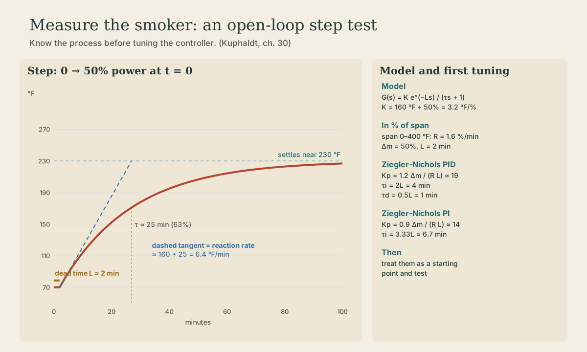
Modeling the smoker from a measured step test: with the controller in manual, a 50 percent power step from 70 °F shows about 2 minutes of dead time, then a first-order rise toward 230 °F with a 25-minute time constant. That gives a first-order-plus-dead-time model, G(s) = 3.2 e^(−2s)/(25s + 1) in °F per percent and minutes; the reaction rate (6.4 °F/min, or 1.6 percent of span per minute); why dead time, not lag, limits how hard you can push; and how too much gain turns control into oscillation.
- 5 min
- 5 steps
- 3 questions
- Lesson 53 of 78
In this lesson
- Know the process first
- Read the model off the curve
- Dead time is the hard part
- Stability
- What to take from this
Picking up where you left off.
Know the process first
Kuphaldt’s first rule of tuning is to understand the process before touching the controller 1. For the smoker, that means a step test: put the controller in manual, hold the element at a fixed output, change it in one step, and record the temperature until it settles. A test like this, with the feedback loop disconnected, is called an open-loop test 1.
Run it on a calm day with the smoker empty and the chip pan in place, logging the grate temperature every few seconds.
Read the model off the curve
Suppose the smoker starts at 70 °F and you step the output from 0 to 50 percent at time zero. The trace shows three things:
- Dead time, L ≈ 2 minutes. Nothing happens at first; the element has to heat up and its heat has to reach the probe.
- First-order rise with time constant τ ≈ 25 minutes. After the dead time the temperature climbs quickly at first and then more slowly, reaching 63 percent of its total change at about 2 + 25 minutes.
- Gain, K. It settles near 230 °F: a 160 °F rise for a 50 percent step, so K = 160 ÷ 50 = 3.2 °F per percent.
A process that settles at a new steady value like this is self-regulating: the smoker loses more heat to the air the hotter it gets, until loss balances input 1.
Those three numbers make a first-order-plus-dead-time model. As a transfer function (with s in 1/minutes):
The steepest slope of the curve, just after the dead time, is the reaction rate: about 160 ÷ 25 = 6.4 °F per minute. Tuning formulas usually want it as a percentage of the measurement span. On a 0–400 °F span, 6.4 °F/min is 1.6 percent per minute 1.
Quick check
Gain is the steady change in output per unit change in input.
Dead time is the hard part
Lag and dead time look similar on a chart but behave very differently in a loop. With lag, the effect of a change starts right away and builds. With dead time, nothing at all happens for a while 1. During those 2 minutes the controller is driving blind: it sees the temperature still low, keeps adding heat, and by the time the effect shows up it has added too much. Kuphaldt puts it bluntly: dead time is a far worse problem for feedback control than lag 1. In the smoker, the ratio that matters is L ÷ τ = 2 ÷ 25: small, which is why it’s an easy loop. Put the probe far from the element and the dead time grows; the loop gets harder.
Playback is optional. If the player is unavailable, open the video at its source.
Quick check
Kuphaldt: dead time is a far worse problem for feedback than lag.
Stability
Close the loop with a proportional controller: output = Kp × error. A larger Kp makes the controller push harder against any error, so the temperature recovers faster. But because of the dead time, each correction arrives late. Push too hard and corrections overshoot, the next one overshoots the other way, and the loop oscillates. A simulation of this smoker model with a controller gain about two and a half times the tuned value from the next lesson kept swinging up and down several degrees around setpoint, never settling. Feedback control is always this trade: enough gain to fight disturbances, not so much that the loop chases its own delayed corrections. MIT’s control course develops the same trade-off formally with poles and stability margins 2.
Quick check
A simulation of this smoker with gain about two and a half times its tuned value never settled.
What to take from this
Measure before you tune: an open-loop step test gives dead time (about 2 min), time constant (about 25 min), and gain (160 °F ÷ 50% = 3.2 °F/%), a first-order-plus-dead-time model G(s) = 3.2e^(−2s)/(25s + 1). The reaction rate is 6.4 °F/min, or 1.6 percent of a 0–400 °F span per minute. Dead time, not lag, is what makes loops hard, and too much gain turns delayed corrections into oscillation.
Lesson complete
Nice work.
Sources for this lesson
- 1Tony R. Kuphaldt. Lessons in Industrial Instrumentation (ch. 21 Continuous Temperature Measurement; ch. 29 Closed-Loop Control; ch. 30 Process Dynamics and PID Controller Tuning). ibiblio.org (Creative Commons Attribution 4.0). verifiedThermocouples: two dissimilar metals produce a temperature-dependent voltage; the junction at the instrument terminals is an unavoidable reference (cold) junction whose voltage must be compensated (example: a type K reading 14.30 mV with terminals at 73 F, which corresponds to 0.910 mV on the NIST ITS-90 table, means a tip voltage of 15.21 mV). Grounded-tip thermocouples respond faster but invite ground loops, so most industrial ones are ungrounded; exposed tips are fastest. The most common failure is open circuit (burnout); with high-impedance inputs an open thermocouple picks up noise from power lines and drives, so instruments need burnout detection. RTDs: platinum, alpha 0.00392, R = R0[1 + alpha(T - T0)]. Process dynamics: know the process before tuning; self-regulating, integrating, and runaway processes need different tuning; dead time (no response at all for a time) is far worse for feedback control than lag. Open-loop (manual) step test: measure dead time L and reaction rate R (max slope, percent per minute) for a step of size delta m; Ziegler-Nichols open-loop: P only Kp = delta m/(R L); PI Kp = 0.9 delta m/(R L), integral time 3.33 L; PID Kp = 1.2 delta m/(R L), integral 2 L, derivative 0.5 L; these are starting points only. Practical controller features: reset (integral) windup when the PV can't reach setpoint no matter how far the output is driven, output limits, manual/automatic modes and output tracking.
- 2Analysis and Design of Feedback Control Systems. MIT OpenCourseWare. verifiedUndergraduate course in transfer functions, time and frequency response, stability, loop shaping, state variables, observers, and digital control.