PID Tuning, Saturation & Digital Implementation
Tuning and coding the smoker's controller: Ziegler-Nichols open-loop starting points from the step test (PID Kp = 1.2Δm/RL ≈ 19 percent per percent, τi = 2L, τd = 0.5L; PI Kp ≈ 14, τi ≈ 6.7 min) converted to °F units, why they're only a start and the final choice is a gentler PI with no derivative, integral windup during preheat (a simulated overshoot to about 290 °F, near the 300 °F fault limit) and the anti-windup fix, output limits, derivative on the measurement, fixed sample time, bumpless manual-to-auto, freezing the integral when the lid opens, and the tests that prove it.
- 5 min
- 6 steps
- 3 questions
- Lesson 54 of 78
In this lesson
- Starting points
- The final tuning
- Integral windup
- Implementation checklist
- Prove it
- What to take from this
Picking up where you left off.
Starting points
The step test (last lesson) gives dead time L = 2 min, reaction rate R = 1.6 percent per minute for an output step of Δm = 50 percent. Ziegler and Nichols’ open-loop rules turn those into tuning settings without even closing the loop 1:
| Controller | Gain Kp | Integral time τi | Derivative time τd |
|---|---|---|---|
| P only | Δm ÷ (R L) ≈ 16 | none | none |
| PI | 0.9 Δm ÷ (R L) ≈ 14 | 3.33 L ≈ 6.7 min | none |
| PID | 1.2 Δm ÷ (R L) ≈ 19 | 2 L = 4 min | 0.5 L = 1 min |
Those gains are in percent of output per percent of measurement span. On a 0–400 °F span, 1 percent is 4 °F, so the PI gain of 14 is 14 ÷ 4 ≈ 3.5 percent output per °F of error. Watch the units: plug a span-based gain into code that computes error in °F and you’ve quadrupled it.
Kuphaldt is clear that these numbers are starting points, not answers 1. The method doesn’t even distinguish self-regulating from integrating processes 1. Start there, then test and back off.
Quick check
With τi = 3.33L ≈ 6.7 minutes; on a 400 °F span that’s about 3.5 percent per °F.
The final tuning
For a smoker, the priorities are no big overshoot (it scorches the outside of the meat and wastes wood), steady holding for hours, and quiet output (less SSR switching noise near the thermocouple). That argues for:
- PI, no derivative. The process is slow and smooth; derivative mostly amplifies measurement noise.
- A gentler gain and slower integral than Ziegler-Nichols: Kp = 2.5 percent per °F (10 percent per percent) and τi = 12 min gave a clean response in simulation of the measured model.
Derivative isn’t wrong in general; for a process with more lag, it can help. If you use it, apply it to the measurement, not the error, so a setpoint change doesn’t kick the output, and filter it.
Quick check
If you use it, take it on the filtered measurement, not the error.
Integral windup
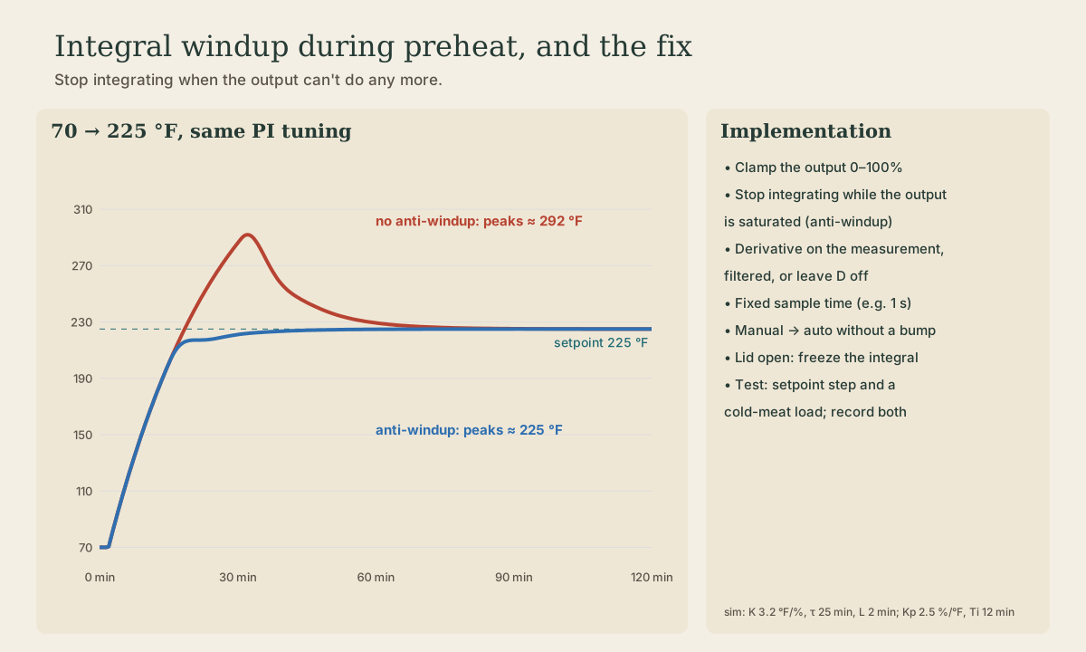
The integral term adds up error over time so the controller eventually removes any steady offset. That’s exactly what causes trouble during preheat. For half an hour the chamber is far below setpoint; the output is pinned at 100 percent and can’t do any more, but the integral keeps accumulating. When the temperature finally reaches setpoint, the integral is enormous, and the controller keeps heating long after it should stop. Kuphaldt describes this as reset windup: the integral grows because the process can’t reach setpoint no matter how far the output is driven 1.
In a simulation of the smoker model with the final tuning, starting the PI at 70 °F with no protection overshot to about 290 °F, close to the 300 °F fault limit, and took the better part of an hour to come back. Two fixes, and the controller uses both:
- Anti-windup: stop integrating whenever the output is saturated at 0 or 100 percent. In the same simulation, the temperature came up to 225 °F with almost no overshoot.
- The PREHEAT state from lesson 4: full power without running the PID until within 20 °F of setpoint, then start the PID with its integral set to a sensible value.
Playback is optional. If the player is unavailable, open the video at its source.
Quick check
Stop integrating while the output is saturated.
Implementation checklist
A digital PID is a few lines of code, and most of the bugs are in the details around it:
- Clamp the output to 0–100 percent, and use output limits deliberately 1.
- Anti-windup: no integration while clamped.
- Fixed sample time: run the loop every second exactly, and scale the integral by the real interval.
- Bumpless transfer: when switching from manual to automatic, start the integral at the current output so it doesn’t jump 1.
- Lid open: a sudden 30-degree drop isn’t something the integral should chase; freeze it until the temperature recovers.
- Faults override everything: any fault (lesson 4) forces the output to 0 regardless of the PID.
Prove it
Test against numbers and keep the logs:
- Setpoint step: hold at 225 °F, step to 250 °F. Target: overshoot under 10 °F, settled within 30 minutes.
- Load disturbance: put in 10 pounds of cold meat. Target: back within 10 °F of setpoint in 20 minutes, without overshooting when it recovers.
- Lid test: open the door for a minute. Target: no overshoot after closing.
- Long hold: a full overnight smoke within ±5 °F at grate level.
MIT’s control course covers the formal tools behind these tests: time and frequency response, stability, and digital control 2.
What to take from this
Ziegler-Nichols open-loop rules turn the step test into starting points (PI: Kp ≈ 14 percent per percent, τi ≈ 6.7 min); convert units carefully (14 per percent of a 400 °F span is 3.5 percent per °F). Then detune for the job: PI, no derivative, Kp 2.5 %/°F, τi 12 min. Prevent integral windup (a simulated 290 °F overshoot without it) by stopping integration while saturated and preheating before the PID starts. Clamp outputs, use a fixed sample time, transfer bumplessly, freeze the integral when the lid opens, and prove it with setpoint, load, and lid tests.
Lesson complete
Nice work.
Sources for this lesson
- 1Tony R. Kuphaldt. Lessons in Industrial Instrumentation (ch. 21 Continuous Temperature Measurement; ch. 29 Closed-Loop Control; ch. 30 Process Dynamics and PID Controller Tuning). ibiblio.org (Creative Commons Attribution 4.0). verifiedThermocouples: two dissimilar metals produce a temperature-dependent voltage; the junction at the instrument terminals is an unavoidable reference (cold) junction whose voltage must be compensated (example: a type K reading 14.30 mV with terminals at 73 F, which corresponds to 0.910 mV on the NIST ITS-90 table, means a tip voltage of 15.21 mV). Grounded-tip thermocouples respond faster but invite ground loops, so most industrial ones are ungrounded; exposed tips are fastest. The most common failure is open circuit (burnout); with high-impedance inputs an open thermocouple picks up noise from power lines and drives, so instruments need burnout detection. RTDs: platinum, alpha 0.00392, R = R0[1 + alpha(T - T0)]. Process dynamics: know the process before tuning; self-regulating, integrating, and runaway processes need different tuning; dead time (no response at all for a time) is far worse for feedback control than lag. Open-loop (manual) step test: measure dead time L and reaction rate R (max slope, percent per minute) for a step of size delta m; Ziegler-Nichols open-loop: P only Kp = delta m/(R L); PI Kp = 0.9 delta m/(R L), integral time 3.33 L; PID Kp = 1.2 delta m/(R L), integral 2 L, derivative 0.5 L; these are starting points only. Practical controller features: reset (integral) windup when the PV can't reach setpoint no matter how far the output is driven, output limits, manual/automatic modes and output tracking.
- 2Analysis and Design of Feedback Control Systems. MIT OpenCourseWare. verifiedUndergraduate course in transfer functions, time and frequency response, stability, loop shaping, state variables, observers, and digital control.