Robot Dynamics, Trajectories & Motion Control

Robot dynamics are often written

The terms represent configuration-dependent inertia, velocity effects, gravity, friction, actuator torque, and external wrench. Stanford’s course progresses from kinematics through Newton-Euler dynamics to joint and operational-space control ¹.

Timing creates force

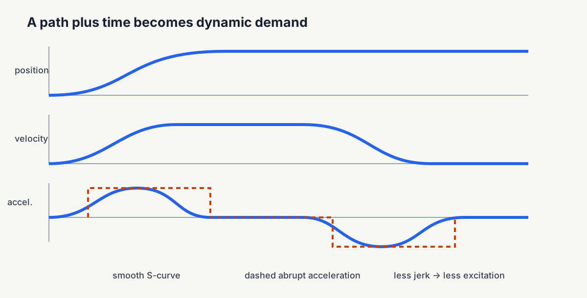
A geometric line can be executed with many time laws. Trapezoidal velocity profiles bound velocity and acceleration but introduce acceleration steps. S-curves bound jerk and often reduce excitation, load shift, and wear. The best cycle time includes motion plus settling, sensing, process time, and recovery—not just commanded travel.

Feedforward and feedback

Feedback corrects mismatch; feedforward supplies predicted gravity, inertia, or friction effort. A joint controller might combine model-based terms with PD error correction. The model reduces routine error; feedback supplies robustness. Neither excuses actuator saturation, delay, calibration, or structural flexibility.

Worked torque screen

A joint sees reflected inertia 0.08 kg·m² and must accelerate at 12 rad/s². Inertial torque is 0.96 N·m. Add worst-case gravity 1.8 N·m, friction 0.25 N·m, and a 20% modeling allowance: roughly \(1.2(0.96+1.8+0.25)=3.61\) N·m before transmission efficiency and dynamic coupling refinement.

Verify across the workspace

Payload torque, Jacobian conditioning, gravity, collision clearance, cable bend, and thermal duty change with pose. Test high-demand corners, not only the convenient center.

Motion study

Plan the same pick move with trapezoidal and S-curve profiles. Compare peak velocity, acceleration, jerk, estimated torque, predicted flexible-mode excitation, and total settle-to-tolerance time. Choose based on good-part cycle time and mechanism life.