Electric Charge, Field, and Gauss's Law

This is the first lesson in electricity and magnetism. It builds on the vector tools you already have, and near the end it leans on two ideas from the math course — the gradient and the divergence theorem — so keep those in mind as you read.

Electric Charge

Electric charge is a fundamental property of matter, much like mass. It comes in two signs, conventionally called positive and negative. Like signs repel; opposite signs attract. Ordinary matter is built from positively charged protons and negatively charged electrons, and an object becomes charged when these are present in unequal numbers ¹.

Three facts about charge organize almost everything that follows. First, charge is conserved: in any closed system the total charge never changes. Charging an object does not create charge out of nothing; it moves existing charge from one place to another. Second, charge is quantized: every observed charge is an integer multiple of a fundamental unit \(e \approx 1.602\times10^{-19}\) coulombs (C), the magnitude of the charge on a single electron or proton. Third, charge is the source of the electric interactions we are about to describe ¹.

Coulomb’s Law

The force between two stationary point charges was measured quantitatively by Charles-Augustin de Coulomb. For two charges \(q_1\) and \(q_2\) separated by a distance \(r\), the magnitude of the force is

Here \(\varepsilon_0\) is the permittivity of free space and \(k \approx 8.99\times10^{9}\ \mathrm{N\cdot m^2/C^2}\). The force points along the line joining the two charges: outward (repulsive) for like signs, inward (attractive) for opposite signs ¹.

Notice the structure. The strength falls off as \(1/r^2\) — the inverse-square law, the same distance dependence as Newtonian gravity — and it grows with the product of the charges. Coulomb’s law is the experimental bedrock of this whole subject.

The Electric Field

Rather than think of charges reaching across empty space to push one another, it is more powerful to say that a charge fills the space around it with an electric field, and that a second charge responds to the field at its own location. The field is defined as force per unit charge. If a small positive test charge \(q\) placed at a point feels a force \(\vec F\), the field there is

\(\vec E=\vec F/q\),

a vector with units of newtons per coulomb (N/C). The field exists whether or not a test charge is there to sample it ¹.

Combining this definition with Coulomb’s law gives the field of a single point charge \(q\). Its magnitude at distance \(r\) is

\(E=\dfrac{kq}{r^2},\)

and it points radially away from the charge when \(q\) is positive and radially toward the charge when \(q\) is negative.

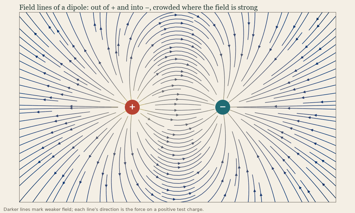
We picture fields with field lines: continuous curves whose direction at each point is the field direction, drawn more densely where the field is stronger. Lines begin on positive charges and end on negative charges.

When several charges are present, the field obeys superposition: the total field at a point is the vector sum of the fields each charge would produce on its own,

This linearity is what makes the subject tractable, because it lets us build the field of any complicated charge arrangement out of simple point-charge contributions ¹.

For a continuous distribution, summation becomes integration, and direct computation can be tedious. The connection to the gradient you saw in the math course hints at a shortcut: an electric field can be written as the gradient of a scalar potential, which often replaces a hard vector integral with an easier scalar one. That potential is taken up in a later lesson.

Gauss’s Law

A second, deeper way to relate field and charge counts the field passing through a closed surface. The electric flux through a surface measures how much field crosses it. Gauss’s law states that the flux through any closed surface equals the charge enclosed, divided by \(\varepsilon_0\):

The left side adds up \(\vec E\cdot d\vec A\) over the whole closed surface, where \(d\vec A\) points outward. The remarkable content is on the right: only the charge enclosed by the surface matters. Charges outside contribute field that enters one side of the surface and leaves the other, netting zero flux ¹.

This is the integral form of one of Maxwell’s equations, and it is exactly where the divergence theorem from vector calculus enters. That theorem equates the flux of a field out of a closed surface with the integral of the field’s divergence over the volume inside. Applying it to Gauss’s law links the surface flux to a local statement about the divergence of \(\vec E\) at each point — the differential form of the same law. The two forms carry the same physics in different clothing.

Gauss’s law is most useful when the charge arrangement has symmetry, because then the field’s direction and magnitude can be argued before any integration. For a uniformly charged sphere, symmetry forces the field to point radially and to depend only on \(r\); choosing a concentric spherical surface then shows that, outside the sphere, the field is identical to that of a point charge holding all the charge at the center. For an infinite charged plane, symmetry makes the field uniform and perpendicular to the plane on each side. In each case symmetry — not heavy calculation — does the work ¹.

Conductors and shielding

Gauss’s law has practical consequences:

• Inside a conductor in equilibrium, the field is zero. Free charges move until they cancel any field inside; any excess charge sits on the outer surface ¹.
• A closed metal shell shields what’s inside. This is the Faraday cage: the mesh in a microwave oven door, shielded cable, and part of why a car body protects its occupants from a lightning strike, since the current flows around the outside.
• Fields crowd at sharp points. Charge concentrates where a conductor curves sharply, so the field is strongest at points and edges. That’s why sparks jump from points and why lightning rods are pointed and grounded.
• Air breaks down at about 3 million V/m. Beyond that, air ionizes and a spark jumps. A static shock that jumps a few millimeters from a fingertip means several thousand volts.