Signals, Noise, Sampling & Conditioning

Microvolts per degree

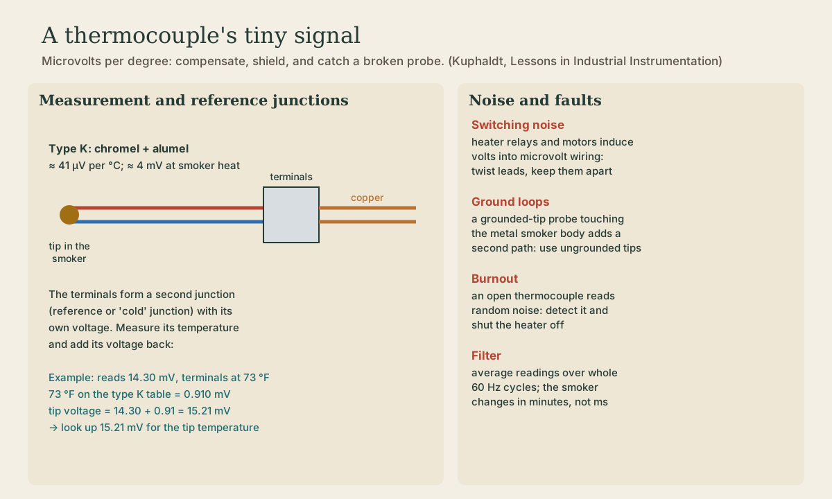
A thermocouple is two wires of different metals joined at the tip. Heat the tip and a small voltage appears between the wires. A type K (chromel and alumel) makes about 41 µV per °C, which is only about 4 mV at smoker temperature. A meter or converter reading it has to resolve a few hundredths of a millivolt to see a single degree, in a box with a 12-amp heater switching on and off a few inches away. Everything in this lesson is about not losing that signal.

The reference junction

There’s a catch built into every thermocouple. Wherever its two wires connect to the instrument’s copper terminals, two more junctions of dissimilar metal form, and they make their own voltage. So a thermocouple doesn’t measure the tip temperature: it measures the difference between the tip and that reference (or cold) junction ¹.

The fix is cold-junction compensation: measure the terminals’ temperature with another sensor and add back the voltage they’re cancelling. Kuphaldt’s worked example: a type K reads 14.30 mV with the terminals at 73 °F. The type K table says a junction at 73 °F makes 0.910 mV, so the tip voltage is 14.30 + 0.91 = 15.21 mV, and that’s the number to look up for the tip temperature ¹. The voltage-to-temperature relationship isn’t linear, which is why tables (the NIST ITS-90 standard) are used instead of a single formula ¹.

In practice, a thermocouple converter chip does both jobs: it measures its own terminal temperature and applies the table internally. Use thermocouple extension wire of the same type all the way to it; ordinary copper wire partway along creates new junctions in the wrong place.

Noise and ground loops

Two things inject noise into a few millivolts:

• Switching: the element’s current and the SSR switching induce voltages in nearby wires. Twist the thermocouple leads together, route them away from the element wiring, and cross power wires at right angles.
• Ground loops: thermocouple probes come with exposed, grounded, or ungrounded tips. A grounded tip is welded to its metal sheath, which responds faster (often less than half the time constant of an ungrounded one) but connects the circuit to whatever the sheath touches, here the smoker’s metal body, forming a ground loop that can add noise and error. That’s why most industrial thermocouples are ungrounded ¹. Use an ungrounded probe; the slower response doesn’t matter in a smoker.

Catch a broken probe

The most common thermocouple failure is the circuit opening, called burnout. An instrument with high input impedance and nothing connected doesn’t read zero: it picks up noise from power lines and motors and reports wild, meaningless temperatures ¹. A good converter detects an open probe and flags it. The controller must treat that flag as a fault: element off. The same goes for a reading that’s impossible (below the outdoor temperature with the element on full for half an hour) or one that jumps 50 degrees in a second.

How often to sample

A smoker’s temperature changes over minutes, not milliseconds; the step test in lesson 5 shows a time constant around 25 minutes. Reading the temperature once a second is plenty. But each reading should be averaged:

• average several conversions per reading to knock down random noise;
• if your converter allows it, average over a whole number of 60 Hz cycles (1/60 s each), so the line-frequency hum cancels instead of aliasing into a slow wander;
• don’t over-filter: a heavy filter adds lag, and lag in the measurement is lag in the control loop.

What to take from this

A type K makes about 41 µV/°C, roughly 4 mV at smoker heat. It measures the tip relative to the terminals, so the terminals’ voltage must be added back (14.30 + 0.91 = 15.21 mV in Kuphaldt’s example); a converter chip and matching extension wire handle it. Twist and separate the leads, use an ungrounded probe to avoid ground loops, detect an open probe and shut the heat off, and sample about once a second with light averaging over whole 60 Hz cycles.