Root Finding and Linear Systems

Two of the most common tasks in numerical computing are finding where a function crosses zero and solving a system of linear equations. Both look like simple algebra problems on paper, but on a computer they become questions about which method to use and how much you can trust the answer. This lesson treats the two themes side by side, building on the calculus and linear algebra you already know.

Root Finding: Solving \(f(x)=0\)

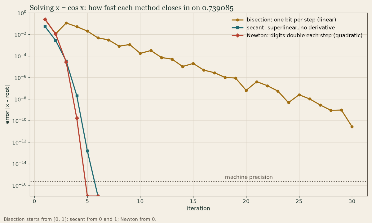
Many problems reduce to finding a value of \(x\) for which some function \(f\) equals zero. Closed-form solutions rarely exist (try solving \(x = \cos x\) by hand), so we use iterative methods that start from a guess and refine it.

Bisection

The most robust method is bisection. It requires a bracket: an interval \([a, b]\) where the function changes sign, so \(f(a)\) and \(f(b)\) have opposite signs. If \(f\) is continuous, the Intermediate Value Theorem guarantees a root lies between them. Each step evaluates \(f\) at the midpoint and keeps whichever half still brackets the sign change. The interval halves every iteration, so the error shrinks by a factor of two each step.

This is linear convergence: reliable but slow. To gain one decimal digit of accuracy you need roughly 3.3 more iterations. Bisection cannot diverge, but it also cannot use any information about the shape of \(f\) to move faster.

Newton’s Method

If you know the derivative, Newton’s method converges much faster. Starting from a guess \(x_n\), it follows the tangent line down to where that line hits zero:

Near a simple root this converges quadratically: the number of correct digits roughly doubles each step. The cost is that you must supply \(f'\), and the method is only locally reliable. A poor starting guess, a derivative near zero, or an inflection point can send the iterates oscillating or diverging entirely. Newton’s method is fast when it works and unforgiving when it does not, which is why a good initial guess matters.

The secant method is a close relative that replaces the exact derivative with a finite-difference slope from the last two iterates, trading a little convergence speed for not needing \(f'\).

Using SciPy

In practice you rarely hand-code these. SciPy’s scipy.optimize module provides robust, well-tested implementations ¹. brentq combines bisection’s safety with faster interpolation and needs only a sign-changing bracket; newton implements Newton’s method (and falls back to the secant method when no derivative is given).

from scipy.optimize import brentq, newton
import numpy as np

f = lambda x: x - np.cos(x)

# Bracketing method: needs an interval where f changes sign
root_brentq = brentq(f, 0.0, 1.0)

# Newton's method: needs a starting guess and (optionally) f'
root_newton = newton(f, x0=0.5, fprime=lambda x: 1 + np.sin(x))

print(root_brentq, root_newton)  # both ~0.739085

Use brentq when you can bracket the root and want a guaranteed answer; reach for newton when you have a good guess and a derivative and want speed.

Worked example: friction in a pipe

The Colebrook equation gives the Darcy friction factor \(f\) for turbulent flow in a pipe, a number every plumbing or pump calculation needs, but \(f\) appears on both sides:

Rearrange to \(g(f) = 0\) and bracket it. For a Reynolds number of 100,000 and relative roughness \(\varepsilon/D = 0.0001\):

import math
from scipy.optimize import brentq

Re, rr = 1e5, 1e-4
g = lambda f: 1 / math.sqrt(f) + 2 * math.log10(rr / 3.7 + 2.51 / (Re * math.sqrt(f)))
f = brentq(g, 0.005, 0.1)
print(round(f, 4))   # 0.0185

Friction factors in turbulent flow fall between roughly 0.008 and 0.1, which makes an easy, safe bracket. The explicit Swamee-Jain approximation gives 0.0185 too, a good check on the root.

Linear Systems: Solving \(A\mathbf{x}=\mathbf{b}\)

Solving \(A\mathbf{x}=\mathbf{b}\) for a square matrix \(A\) is the workhorse of scientific computing. From your linear algebra course you already know the right conceptual tool: Gaussian elimination, the systematic process of using row operations to reduce \(A\) to triangular form and then back-substituting.

Numerical solvers do exactly this, organized as LU factorization. The matrix is decomposed once into a lower-triangular factor \(L\) and an upper-triangular factor \(U\) (with row pivoting for stability), so that \(A = LU\). Solving then becomes two fast triangular solves: \(L\mathbf{y} = \mathbf{b}\) followed by \(U\mathbf{x} = \mathbf{y}\). This is the same elimination you learned, just bookkept so the expensive factorization can be reused across many right-hand sides.

Solve Directly; Do Not Invert

The single most important rule carries straight over from linear algebra: solve the system directly rather than forming the inverse ². It is tempting to write \(\mathbf{x} = A^{-1}\mathbf{b}\), but computing \(A^{-1}\) and then multiplying does strictly more arithmetic than elimination and accumulates more rounding error. Just as you would not invert a matrix by hand to solve a small system, you should let the computer eliminate.

In NumPy, that means numpy.linalg.solve(A, b), never numpy.linalg.inv(A) @ b:

import numpy as np

A = np.array([[3.0, 2.0, -1.0],
              [2.0, -2.0, 4.0],
              [-1.0, 0.5, -1.0]])
b = np.array([1.0, -2.0, 0.0])

x = np.linalg.solve(A, b)        # direct solve via LU factorization
print(x)
print(np.allclose(A @ x, b))     # True: x satisfies the system

numpy.linalg.solve performs the LU factorization and triangular solves internally and is both more accurate and more efficient than inverting. If you ever genuinely need the same \(A\) solved against dozens of different \(\mathbf{b}\) vectors, the right move is still to factor once (e.g., with scipy.linalg.lu_factor/lu_solve) rather than to invert.

Takeaways

Root finding gives you a tradeoff between safety and speed: bisection always converges but slowly, Newton’s method converges quadratically but can fail without a good guess and a derivative, and library routines like brentq and newton package the robust choices. For linear systems, lean on the elimination intuition you already have, let LU-based solvers do the work, and always prefer a direct solve over forming an inverse.