Integration and the Fundamental Theorem

From Rates to Totals

Earlier lessons treated the derivative as an instrument for measuring instantaneous rates of change. Integration runs the machinery in reverse. Where differentiation breaks a quantity into its moment-to-moment rate, integration accumulates a rate back into a total. If a derivative answers “how fast?”, an integral answers “how much, all together?” These two ideas turn out to be inverses of one another, and the precise statement of that relationship is the central result of this lesson ¹.

The Definite Integral as a Limit of Riemann Sums

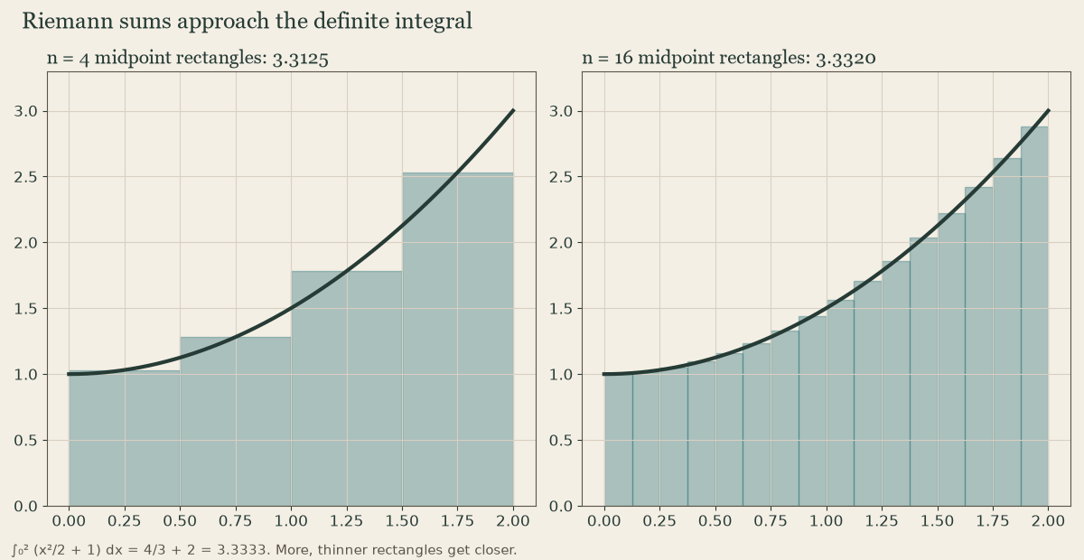
Suppose you want the area under the curve \(y=f(x)\) between \(x=a\) and \(x=b\). Slice the interval \([a,b]\) into \(n\) equal subintervals of width \(\Delta x=(b-a)/n\). On each subinterval pick a sample point \(x_i^*\) and build a rectangle of height \(f(x_i^*)\). Summing the rectangles gives a Riemann sum, an approximation that sharpens as the rectangles narrow. The definite integral is the limit of these sums:

When this limit exists, \(f\) is said to be integrable on \([a,b]\); every continuous function is ¹. The result is a signed area: regions above the \(x\)-axis count positively, regions below count negatively. More generally, the integral accumulates whatever quantity \(f\) represents. If \(f\) is a velocity, the integral is a net displacement; if \(f\) is a flow rate, it is a total volume.

The Indefinite Integral and the Constant of Integration

A function \(F\) is an antiderivative of \(f\) if \(F'(x)=f(x)\). Because the derivative of any constant is zero, antiderivatives are never unique: if \(F\) works, so does \(F(x)+C\) for any constant \(C\). The whole family is written as the indefinite integral,

The “\(+C\)” is not decoration; it records the fact that infinitely many functions share the same derivative, differing only by a vertical shift. The indefinite integral names a family of functions, whereas the definite integral produces a single number.

Basic Antiderivatives

Reversing the differentiation rules gives a starter table ¹:

• Power rule: \(\displaystyle\int x^{n}\,dx=\frac{x^{n+1}}{n+1}+C\) for \(n\neq-1\).
• Exponential: \(\displaystyle\int e^{x}\,dx=e^{x}+C\).
• Reciprocal (the \(n=-1\) case): \(\displaystyle\int \frac{1}{x}\,dx=\ln|x|+C\).
• Trigonometric: \(\displaystyle\int \cos x\,dx=\sin x+C\) and \(\displaystyle\int \sin x\,dx=-\cos x+C\).

Each entry is just a derivative read backward, which is why fluency with differentiation pays off immediately here.

Properties That Make Integrals Manageable

Two structural properties let you break complicated integrals into simpler pieces ¹. Linearity says integration respects sums and constant multiples:

Additivity over intervals says you can split the domain and add the parts:

A useful companion convention is that reversing the limits flips the sign: \(\int_b^a f(x)\,dx=-\int_a^b f(x)\,dx\), so \(\int_a^a f(x)\,dx=0\).

The Fundamental Theorem of Calculus

The Fundamental Theorem of Calculus (FTC) welds differentiation and integration into a single inverse relationship, and it comes in two parts ¹.

Part 1 considers the area-so-far function \(g(x)=\int_a^x f(t)\,dt\), which records accumulated area from the fixed point \(a\) out to a moving endpoint \(x\). For continuous \(f\),

Differentiating an accumulation hands back the original integrand. In words: the rate at which accumulated area grows is exactly the height of the curve at the leading edge.

Part 2 turns that insight into a computational tool. If \(F\) is any antiderivative of \(f\) on \([a,b]\), then

This is the engine of practical integration: rather than evaluating a limit of Riemann sums directly, find an antiderivative and subtract its values at the endpoints. Part 1 guarantees such an antiderivative exists for continuous functions; Part 2 shows how to use it. Together they explain why the two operations are genuine inverses, accumulation undoing rate and rate undoing accumulation.

A Worked Evaluation

Compute \(\displaystyle\int_1^3 x^2\,dx\). An antiderivative of \(x^2\) is \(F(x)=\tfrac{x^3}{3}\). By Part 2,

The constant \(C\) is omitted deliberately: it appears in both \(F(3)\) and \(F(1)\) and cancels in the subtraction, which is why any antiderivative will do.

Why Engineers Care

For engineering work the integral is the standard way to convert a rate into a total. Integrating a velocity over time yields distance traveled; integrating a power curve yields energy delivered; integrating a load distribution along a beam yields total force, and integrating that yields bending moment. The recurring pattern is total accumulated change equals the integral of the rate of change ¹. Whenever a measured signal represents how fast something happens, integration recovers how much of it has happened, and the Fundamental Theorem makes that recovery a matter of evaluating an antiderivative at two endpoints.