Multiple Integrals

A single-variable definite integral \(\int_a^b f(x)\,dx\) accumulates a quantity along an interval — most familiarly, the signed area under a curve. Multiple integrals extend that same accumulation idea to functions of two or more variables, letting you measure volumes, total mass, and averages over regions of the plane or space. If you are comfortable with definite integrals and partial derivatives, the leap is smaller than it looks: a multiple integral is still a limit of sums, just over a region instead of an interval.

The Double Integral

For a function \(f(x,y)\) defined on a region \(R\) in the plane, the double integral is written

Geometrically, when \(f\ge 0\), this is the volume of the solid lying above \(R\) and below the surface \(z=f(x,y)\). The construction mirrors the single-variable case: partition \(R\) into small pieces of area \(\Delta A\), pick a sample point \((x_i,y_i)\) in each, form the sum \(\sum_i f(x_i,y_i)\,\Delta A\) of box volumes, and take the limit as the pieces shrink ¹. More generally, \(\iint_R f\,dA\) is the accumulated value of \(f\) over the region, whatever \(f\) represents physically.

Iterated Integrals and Fubini’s Theorem

Evaluating that limit directly is impractical. Fubini’s theorem rescues us: over a rectangle \(R=[a,b]\times[c,d]\), the double integral equals an iterated integral, computed one variable at a time,

Work from the inside out. The inner integral \(\int_c^d f(x,y)\,dy\) treats \(x\) as a constant and integrates in \(y\), producing a function of \(x\); the outer integral then integrates that result in \(x\). When \(f\) is continuous, the order may be swapped (integrate in \(x\) first, then \(y\)) without changing the answer ¹. Notice the symmetry with partial differentiation: just as \(\partial/\partial y\) holds \(x\) fixed, the inner integral integrates in \(y\) with \(x\) held fixed.

Non-Rectangular Regions

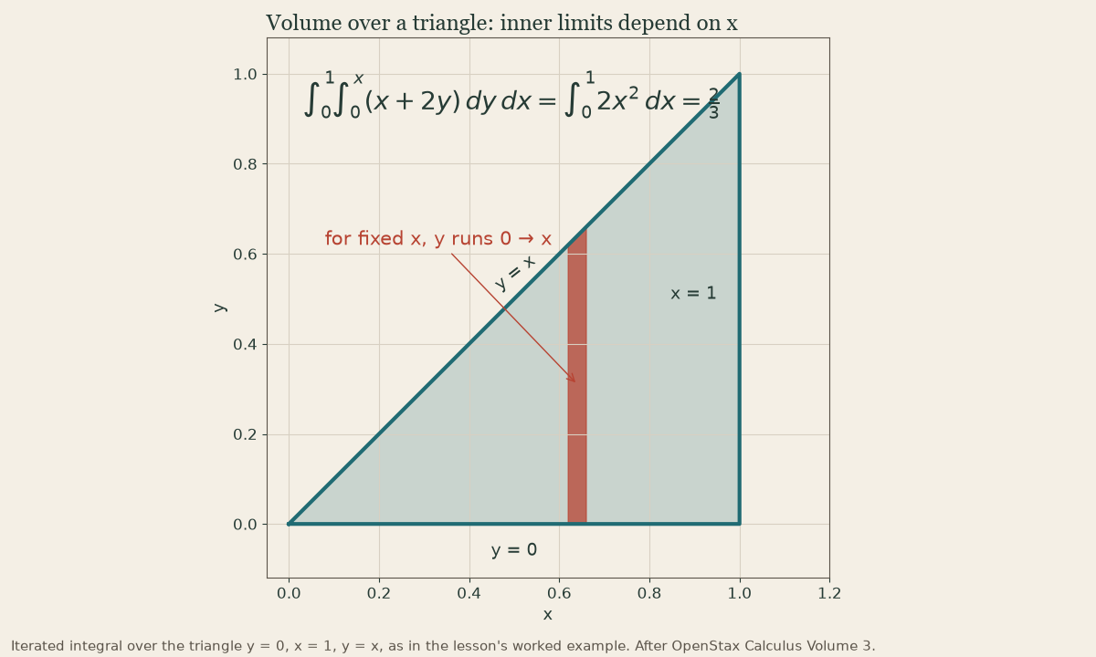
Real regions are rarely rectangles. If \(R\) is bounded below and above by curves \(y=g_1(x)\) and \(y=g_2(x)\) for \(x\) in \([a,b]\), the inner limits become functions of \(x\):

The inner (variable) limits describe how the region’s vertical extent changes as \(x\) moves; the outer (constant) limits sweep across the region. Sketching \(R\) first is the surest way to read off correct limits ¹.

A Worked Example

Find the volume under \(f(x,y)=x+2y\) over the triangle \(R\) bounded by \(y=0\), \(x=1\), and \(y=x\). For a fixed \(x\) in \([0,1]\), \(y\) runs from \(0\) up to \(x\):

Inner integral in \(y\):

Outer integral in \(x\):

The volume is \(2/3\). A useful check: integrating the constant function \(f=1\) over \(R\) gives the area of \(R\), here \(\tfrac12\), confirming the limits describe the intended triangle.

Triple Integrals

The same logic extends to three variables. For \(f(x,y,z)\) over a solid region \(E\),

is evaluated as a triply iterated integral, with the innermost limits possibly depending on the outer variables. Setting \(f=1\) yields the volume of \(E\); a general \(f\) accumulates that quantity throughout the solid ¹.

Changing Coordinates

When a region or integrand has circular symmetry, polar coordinates simplify the work. Substituting \(x=r\cos\theta\), \(y=r\sin\theta\), the area element is not \(dr\,d\theta\) but

so \(\iint_R f\,dA=\iint f(r\cos\theta,r\sin\theta)\,r\,dr\,d\theta\). The extra factor \(r\) accounts for the fact that polar “grid cells” grow wider as they move away from the origin ¹. For triple integrals, cylindrical coordinates add a \(z\)-axis (element \(r\,dr\,d\theta\,dz\)) and spherical coordinates suit ball-like regions (element \(\rho^2\sin\phi\,d\rho\,d\phi\,d\theta\)).

These factors are instances of one idea: the Jacobian. Any change of variables \((x,y)=T(u,v)\) rescales area by the absolute value of the determinant of the matrix of partial derivatives, \(\left|\partial(x,y)/\partial(u,v)\right|\), so \(dA=\left|\partial(x,y)/\partial(u,v)\right|\,du\,dv\). For polar coordinates that determinant works out to exactly \(r\) ¹.

Why Engineers Care

Multiple integrals turn local quantities into totals. If \(\rho(x,y)\) is a surface mass density, the total mass of a plate is \(\iint_R \rho\,dA\); for a solid of density \(\rho(x,y,z)\), the mass is \(\iiint_E \rho\,dV\). Setting density to \(1\) recovers pure area or volume. The centroid (center of mass) follows from density-weighted integrals such as \(\bar{x}=\frac{1}{M}\iint_R x\,\rho\,dA\). These centroid and mass computations feed directly into statics — locating centers of gravity, computing distributed loads, and (with an extra distance-squared factor) moments of inertia.