Sensors, Metrology & Uncertainty
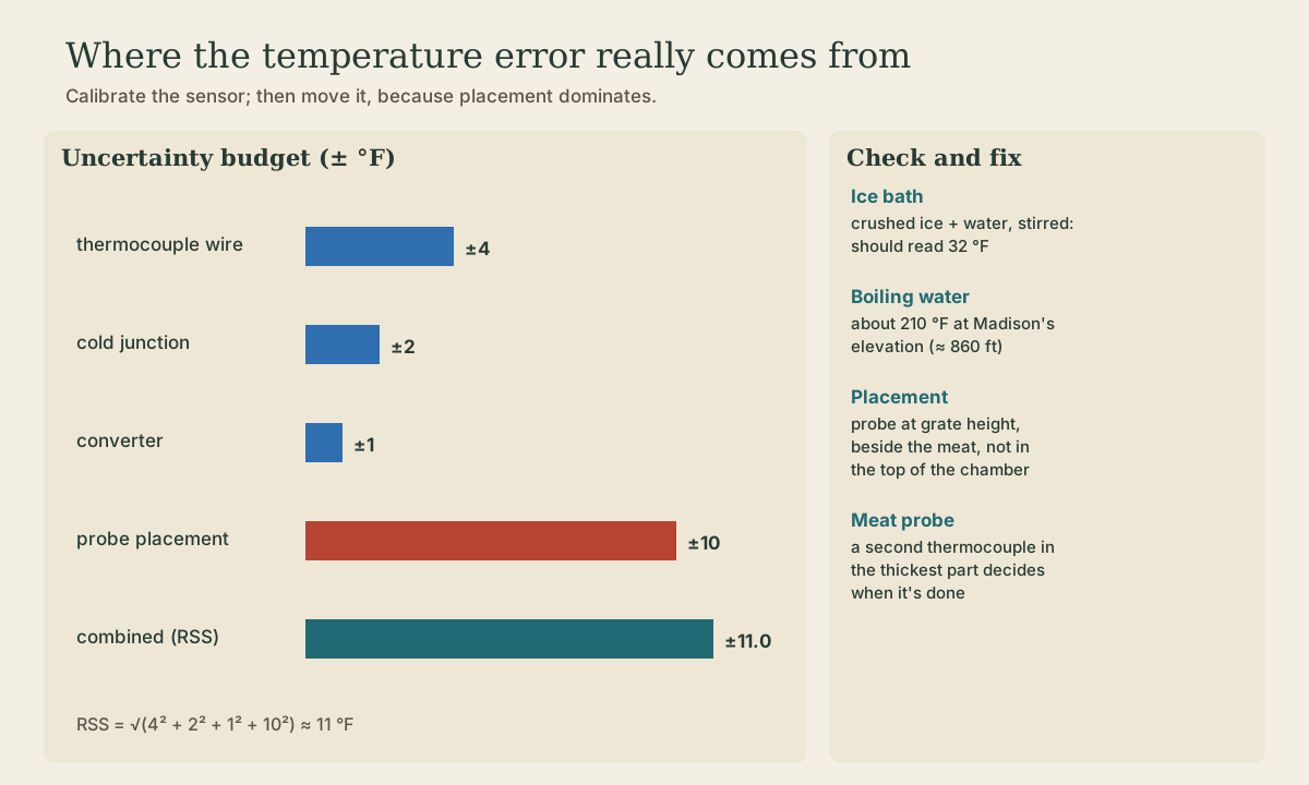
Choosing and trusting the smoker's temperature sensors: thermocouples versus RTDs (R = R₀[1 + α(T − T₀)], α = 0.00392 for platinum) versus thermistors; a worked uncertainty budget (thermocouple wire ±4 °F, cold junction ±2, converter ±1, probe placement ±10, root-sum-square about ±11 °F) that shows placement dominates; two-point checks in ice water and boiling water corrected for Madison's elevation; response time; and why the meat probe, not the chamber probe, decides when it's done.
- 4 min
- 6 steps
- 3 questions
- Lesson 51 of 78
In this lesson
- Thermocouple, RTD, or thermistor
- Build the budget
- Check it against something you know
- Response time
- Which probe decides
- What to take from this
Picking up where you left off.
Thermocouple, RTD, or thermistor
Three common sensors could do the job:
- Thermocouple (type K): cheap, rugged, wide range, thin and fast; needs cold-junction compensation and careful wiring (last lesson).
- RTD (resistance temperature detector): a platinum wire whose resistance rises with temperature, roughly R = R₀[1 + α(T − T₀)]. With α = 0.00392 for typical platinum, a 100 Ω RTD reads 100[1 + 0.00392 × 35] = 113.72 Ω at 35 °C 1. More accurate and stable than a thermocouple, but bulkier, pricier, and slower.
- Thermistor: a ceramic bead with a large resistance change over a narrow range; very sensitive, very non-linear, and many types don’t tolerate smoker heat for long.
For a smoker, a thermocouple wins on ruggedness and price, as long as you know how much to trust it.
Quick check
R = 100[1 + 0.00392 × 35] = 113.72 Ω (Kuphaldt’s example).
Build the budget
Every reading has several independent sources of error. Estimate each, then combine them. For independent errors, add the squares and take the square root (root-sum-square):
| Source | ± °F |
|---|---|
| Thermocouple wire (standard grade type K, about ±2.2 °C) | 4 |
| Cold-junction compensation | 2 |
| Converter | 1 |
| Probe placement: chamber temperature varies from the top to the grate, near the element versus near the door | 10 |
| Combined (√(4² + 2² + 1² + 10²)) | ≈ 11 |
The sensor chain contributes about ±4.6 °F combined; where the probe sits contributes ±10. Spending money on a better sensor barely changes the total. Moving the probe to grate height, next to the meat, does. This is the usual lesson of a measurement budget: the biggest term is often not the instrument.
Quick check
RSS of 4, 2, 1, and 10 is about 11: fixing placement matters most.
Check it against something you know
Two easy reference points:
- Ice bath: fill a glass with crushed ice, add water, stir, wait a minute. It should read 32 °F.
- Boiling water: water boils at 212 °F at sea level, but lower as elevation rises and air pressure drops, roughly 1 °F lower per 500 feet. Madison sits around 860 feet, so expect about 210 °F.
If both readings are off by the same amount, add an offset in the controller. If they’re off by different amounts, the problem is probably the probe or its wiring, not something an offset should hide.
Quick check
Correct the reference point before you correct the sensor.
Response time
A sensor doesn’t report a change instantly. A probe’s time constant is how long it takes to show about 63 percent of a sudden change. Bare (exposed) tips are fastest, grounded tips next, ungrounded tips slowest, often by a factor of two or more 1. In a smoker with a 25-minute time constant, an ungrounded probe’s few seconds of lag don’t matter. In the control loop of a fast process, they would.
Which probe decides
The chamber probe controls the heat, but it doesn’t say when the food is done. A second thermocouple in the thickest part of the meat does. The bacon method, for example, smokes at 225–250 °F until the bacon reaches 160 °F inside 2. The controller’s job ends when the meat probe says so, not when a timer runs out. That probe needs its own check in ice water and boiling water.
What to take from this
Thermocouples suit smokers (rugged, cheap, wide range); RTDs are more accurate (R = R₀[1 + αΔT], α = 0.00392); thermistors are sensitive over narrow ranges. Build a root-sum-square budget: here ±4, 2, 1, and 10 °F combine to about ±11, and placement dominates. Check probes in ice water (32 °F) and boiling water (about 210 °F in Madison). Put the chamber probe at grate height beside the meat, and let the meat probe (160 °F for bacon) decide when it’s done.
Lesson complete
Nice work.
Sources for this lesson
- 1Tony R. Kuphaldt. Lessons in Industrial Instrumentation (ch. 21 Continuous Temperature Measurement; ch. 29 Closed-Loop Control; ch. 30 Process Dynamics and PID Controller Tuning). ibiblio.org (Creative Commons Attribution 4.0). verifiedThermocouples: two dissimilar metals produce a temperature-dependent voltage; the junction at the instrument terminals is an unavoidable reference (cold) junction whose voltage must be compensated (example: a type K reading 14.30 mV with terminals at 73 F, which corresponds to 0.910 mV on the NIST ITS-90 table, means a tip voltage of 15.21 mV). Grounded-tip thermocouples respond faster but invite ground loops, so most industrial ones are ungrounded; exposed tips are fastest. The most common failure is open circuit (burnout); with high-impedance inputs an open thermocouple picks up noise from power lines and drives, so instruments need burnout detection. RTDs: platinum, alpha 0.00392, R = R0[1 + alpha(T - T0)]. Process dynamics: know the process before tuning; self-regulating, integrating, and runaway processes need different tuning; dead time (no response at all for a time) is far worse for feedback control than lag. Open-loop (manual) step test: measure dead time L and reaction rate R (max slope, percent per minute) for a step of size delta m; Ziegler-Nichols open-loop: P only Kp = delta m/(R L); PI Kp = 0.9 delta m/(R L), integral time 3.33 L; PID Kp = 1.2 delta m/(R L), integral 2 L, derivative 0.5 L; these are starting points only. Practical controller features: reset (integral) windup when the PV can't reach setpoint no matter how far the output is driven, output limits, manual/automatic modes and output tracking.
- 2Joy Waite-Cusic, Jared Hibbard-Swanson. Making Cured Bacon at Home (PNW 784). Oregon State University Extension. 2025. verifiedDry cure or wet brine; Prague Powder #1 is 6.25 percent sodium nitrite and 93.75 percent salt, dyed pink and not the same as Himalayan pink salt; 1 teaspoon per 5 pounds of meat; dry-cured bacon is capped at 200 ppm nitrite commercially; Cure #2 not recommended for bacon (nitrosamines at high heat); cure 5-7 days at 40 F, flipping daily; smoke at 225-250 F to 160 F internal; refrigerate up to 7 days, freeze within 4 months.