Inverse Kinematics, Jacobians & Singularities

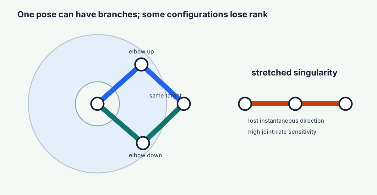
Inverse kinematics (IK) asks which joint configurations produce a desired tool pose. There may be no solution, one boundary solution, several branches, or infinitely many for a redundant robot.

Stanford CS223A places inverse kinematics after spatial descriptions and forward kinematics, then connects it to Jacobians, dynamics, and control ¹. That order matters: IK is not a free-standing angle solver. It depends on the frame definitions, tool transform, joint convention, limits, and geometry already established.

For the planar two-link arm, distance \(r=\sqrt{x^2+y^2}\) must satisfy

The law of cosines gives

typically yielding elbow-up and elbow-down branches. Select using joint limits, collision, cable routing, stiffness, continuity from current pose, and downstream task—not angle size alone.

The corresponding shoulder solution is

Worked two-link solution

Let \(l_1=0.40\) m, \(l_2=0.30\) m, and target \((x,y)=(0.40,0.30)\) m. Here \(r=0.50\) m and

Therefore \(q_2=+90^\circ\) or \(-90^\circ\). Substitution gives approximately \((q_1,q_2)=(0^\circ,90^\circ)\) and \((73.7^\circ,-90^\circ)\). Both reach the point. Joint limits, obstacles, approach direction, and continuity decide which is usable. Re-run forward kinematics on every returned solution; it is the cheapest sign and convention check.

The Jacobian

For joint vector \(q\) and task velocity \(\dot x\),

Static wrench relationship is \(\tau=J^T F\). The same geometry that maps velocity maps force in a dual way. Near a singularity, modest Cartesian velocity can require extreme joint speed, and some force directions become weak or uncontrollable.

For the planar two-link position task,

and \(\det J=l_1l_2\sin q_2\). The arm loses rank when \(q_2=0\) or \(\pi\): the links are collinear. Determinant is useful for this square example, but singular values generalize better to non-square and higher-dimensional Jacobians.

The smallest singular value measures the weakest instantaneous task direction. Condition number compares strongest with weakest amplification. Always define units and scaling when rotation and translation share a task vector; changing meters to millimeters otherwise changes the numerical condition measure.

Singularity-aware planning

Watch Jacobian rank, determinant for square cases, singular values, or condition number. Set operational thresholds before numerical inversion becomes explosive. Damped least squares trades perfect task tracking for bounded joint motion near singularity.

One common velocity form is

Larger damping \(\lambda\) bounds joint speed but increases task error. Use a documented schedule tied to a singular-value threshold, cap joint rate and acceleration, and test the resulting path rather than relying on numerical convergence alone. The Stanford archive provides lectures, notes, and assignments that make these kinematic and differential relationships worth practicing by hand before hiding them in a solver ².

For a redundant robot, a null-space term can pursue a secondary objective without changing the commanded task velocity in the local linear model. Joint-limit avoidance, posture, manipulability, collision clearance, and cable management are possible objectives, but competing weights can cause discontinuities or unexpected posture changes.

Workspace is more than reach

Separate reachable position workspace, dexterous workspace with required orientations, payload-rated workspace, collision-free workspace, and process-qualified workspace. A catalog reach sphere does not prove the robot can weld, insert, or inspect at every point within it.

Make IK a planning service

A production-quality IK request should include target frame and timestamp, tool and payload configuration, seed posture, joint and velocity limits, collision model, approach constraints, tolerances, and timeout. The result should report branch, residual error, margins, condition measure, collision status, and failure reason.

Prefer branch continuity along a path. Solving independent points with no seed can jump between elbow branches even when each pose is valid. Interpolate and validate the whole motion, including swept volume, joint speed and acceleration, singularity margin, and process orientation. MIT’s robotics course reinforces this integration of mechanisms, kinematics, planning, control, sensing, and projects ³.

Solver acceptance set

Test reachable and unreachable targets, boundary poses, multiple branches, joint-limit contact, near-singular motion, collision, stale frames, bad calibration, changed tool, and restart from a different seed. Preserve both successful solutions and structured failure codes. “No solution” must be distinguishable from timeout, collision rejection, numerical failure, or an invalid frame.

Exercise

For a two-link arm, plot or tabulate five target points. Solve both IK branches, check joint limits, calculate a Jacobian condition measure, and choose one configuration with a written rationale. Add a keep-out region and see whether the best kinematic branch changes.

After solving the five points, connect them as a path. Seed each solve from the previous configuration, graph joint rates, and mark the minimum singular value. Compare plain pseudoinverse and damped least squares near the worst point, including task error and peak joint speed.