Searching and Big-O
Linear search checks every item; binary search, on sorted data, halves the possibilities with each check, so ten million items take 24 checks instead of ten million. Logarithms as repeated halving; big-O notation, which keeps how an algorithm's time grows and drops the details, with its hierarchy from O(1) to O(2^n) and a table of what each means for a million items; worst and average cases; the doubling test, which tells you an algorithm's growth from two timings; and binary search in practice, with Python's bisect module and git bisect.
- 10 min
- 8 steps
- 3 questions
- Lesson 78 of 80
In this lesson
- Two ways to search
- Logarithms
- Big-O
- Worst case and average case
- The doubling test
- Binary search in practice
- Your turn
- So
Picking up where you left off.
Two ways to search
To find something in a list, the obvious method is linear search: check the first item, then the next, and so on. If the item is last, or missing, that’s every item checked.
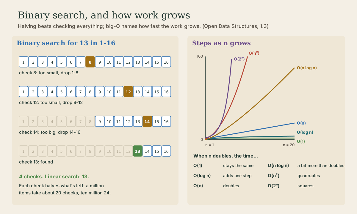
If the list is sorted, there’s a much better way. Binary search checks the middle item. If that’s too small, the target can only be in the upper half, so the lower half is discarded; if it’s too big, the upper half goes. Each check halves what’s left, so for n items it needs at most about log₂ n checks 1. It’s how you’d look up a word in a paper dictionary, or guess a number between 1 and 100 when told “higher” or “lower.”
This program counts the checks each method makes to find the last item. Save it as search.py:
# search.py: count the comparisons linear search and binary search make.

def linear_search(items, target):
    """Check each item in turn."""
    for count, item in enumerate(items, start=1):
        if item == target:
            return count
    return len(items)

def binary_search(items, target):
    """Items must be sorted. Check the middle, then throw away the half that can't hold target."""
    lo, hi, count = 0, len(items) - 1, 0
    while lo <= hi:
        mid = (lo + hi) // 2
        count += 1
        if items[mid] == target:
            return count
        if items[mid] < target:
            lo = mid + 1                # target is in the upper half
        else:
            hi = mid - 1                # target is in the lower half
    return count

for n in (1_000, 1_000_000, 10_000_000):
    items = range(n)                    # sorted, and indexable without storing every number
    target = n - 1                      # the last item: the worst case for a linear search
    print(f"n = {n:>10,}   linear: {linear_search(items, target):>10,} checks   binary: {binary_search(items, target):>2} checks")
lo and hi mark the part of the list that could still hold the target; each pass through the loop moves one of them past the middle.
me@linuxbox:~$ python3 search.py
n =      1,000   linear:      1,000 checks   binary: 10 checks
n =  1,000,000   linear:  1,000,000 checks   binary: 20 checks
n = 10,000,000   linear: 10,000,000 checks   binary: 24 checks
Multiplying the data by ten thousand took binary search from 10 checks to 24.
Quick check
2^20 is about a million, so twenty halvings narrow a million possibilities to one.
Logarithms
The logarithm base 2, log₂ n, answers: how many times can you halve n before you get down to 1 1? log₂ 1,000 is about 10, log₂ 1,000,000 about 20, and log₂ 1,000,000,000 about 30. Doubling n adds just one to it. That’s why anything that halves its problem at each step, binary search, a balanced search tree, scales so well.
Big-O
Counting exact steps is hopeless: the real time depends on the machine, the language, and a dozen constants nobody knows 1. Big-O notation keeps only how the time grows with the size of the input, n. A function f(n) is O(g(n)) if, for all large enough n, f(n) is at most some constant times g(n) 1. In practice that means: keep the fastest-growing term and drop constant factors. A running time of 5n log n + 8n − 200 is O(n log n) 1.
The common classes, from best to worst 1:
| Big-O | Name | Example |
|---|---|---|
| O(1) | constant | items[k], x in a_set |
| O(log n) | logarithmic | binary search |
| O(n) | linear | linear search, x in a_list |
| O(n log n) | “n log n” | good sorting algorithms (next lesson) |
| O(n²) | quadratic | comparing every item with every other; n inserts at a list’s front |
| O(2ⁿ) | exponential | trying every subset of n items |
The differences get enormous. This program prints the step counts for a few sizes. Save it as growth_table.py:
# growth_table.py: how many steps each kind of algorithm takes as n grows.
import math

print(f"{'n':>9}  {'log2 n':>6}  {'n log2 n':>12}  {'n^2':>17}  {'2^n':>12}")
for n in (10, 100, 1_000, 1_000_000):
    print(f"{n:>9,}  {math.log2(n):>6.1f}  {round(n * math.log2(n)):>12,}  {n * n:>17,}  "
          f"{'about 10^' + str(round(n * math.log10(2))):>12}")
me@linuxbox:~$ python3 growth_table.py
        n  log2 n      n log2 n                n^2           2^n
       10     3.3            33                100    about 10^3
      100     6.6           664             10,000   about 10^30
    1,000    10.0         9,966          1,000,000  about 10^301
1,000,000    19.9    19,931,569  1,000,000,000,000  about 10^301030
At a billion simple steps a second, a million items take: about 20 nanoseconds at O(log n), a millisecond at O(n), 0.02 seconds at O(n log n), and 1,000 seconds, nearly 17 minutes, at O(n²) 1. At O(2ⁿ), even n = 100 would take about 40 trillion years.
Big-O is a statement about large n. If two algorithms have different big-O, the one with the smaller growth wins once n is big enough; if they have the same big-O, only measuring tells you which is faster, and the answer may differ between machines 1. An O(n) algorithm taking 15n steps loses to an O(n log n) one taking 2n log₂ n steps until n passes about 181 1, and then wins by more and more.
Quick check
Big-O ignores constant factors: 15n is more than 2n log₂ n until n passes about 181.
Worst case and average case
Big-O usually describes the worst case, unless it says otherwise. Linear search’s worst case is n checks; on average, for a target that’s present, it’s about n/2, which is still O(n). Some structures are quoted by their average case: a dict lookup is O(1) on average and O(n) in the worst case, when every key collides 2. Last module’s binary search tree was the same story: about 12 visits among 1,000 random keys, 500 on average for sorted ones.
The doubling test
You can often read an algorithm’s growth straight from its timings: run it at size n, then at 2n, and compare. Here are three ways to ask “is x here?” timed at three sizes. Save it as doubling.py:
# doubling.py: double n and watch how each kind of lookup's time changes.
import time
from bisect import bisect_left

def per_lookup(fn, repeats):
    start = time.perf_counter()
    for _ in range(repeats):
        fn()
    return (time.perf_counter() - start) / repeats * 1e6      # microseconds

print(f"{'n':>10}  {'x in list':>12}  {'bisect':>9}  {'x in set':>9}   (microseconds)")
for n in (1_000_000, 2_000_000, 4_000_000):
    items = list(range(n))
    as_set = set(items)
    x = n - 1
    scan = per_lookup(lambda: x in items, 20)                  # O(n)
    halve = per_lookup(lambda: bisect_left(items, x), 100_000) # O(log n)
    hashed = per_lookup(lambda: x in as_set, 100_000)          # O(1)
    print(f"{n:>10,}  {scan:>12.1f}  {halve:>9.3f}  {hashed:>9.3f}")
On a desktop PC:
me@linuxbox:~$ python3 doubling.py
         n     x in list     bisect   x in set   (microseconds)
 1,000,000        3038.5      0.120      0.029
 2,000,000        6201.4      0.109      0.029
 4,000,000       12243.7      0.121      0.047
The list scan doubles each time: O(n). Binary search barely moves, since doubling n adds one check to about twenty: O(log n). The set stays tiny: O(1), give or take some noise from the memory hierarchy. The general rule:
| When n doubles, the time… | Big-O |
|---|---|
| stays the same | O(1) |
| grows by a constant step | O(log n) |
| doubles | O(n) |
| a bit more than doubles | O(n log n) |
| quadruples | O(n²) |
| squares | O(2ⁿ) |
Last module’s list.insert(0, x) loop went from 1.0 to 3.9 seconds when n doubled: four times, so the whole loop was O(n²).
Quick check
(2n)² = 4n². An O(n) program would only double, and O(4n) is just O(n).
Binary search in practice
Python’s bisect module does binary search on sorted lists. bisect_left(a, x) returns the position where x would go to keep a sorted, which is also where x is if it’s present 3. The module’s documentation shows how to build exact lookups from it 3:
from bisect import bisect_left

def index(a, x):
    'Locate the leftmost value exactly equal to x'
    i = bisect_left(a, x)
    if i != len(a) and a[i] == x:
        return i
    raise ValueError
Binary search needs sorted data, and keeping data sorted has its own cost; that’s next lesson. And you’ve used binary search before: git bisect (Git course) finds the commit that introduced a bug by testing the commit halfway between a known good one and a known bad one, then halving again 4. A thousand commits take about ten tests.
Your turn
Exercises
- How many checks would binary search need, at most, for a billion sorted items? For ten billion?
- In
search.py, change the target to0, the first item. How many checks does each method make now? - Simplify to big-O:
3n² + 100n + 7;50 log n + 4;n(n − 1)/2;1000. - A script takes 2 seconds on a 10,000-line file and 8 seconds on a 20,000-line file. What’s its likely big-O, and how long would 40,000 lines take?
- Write
contains(a, x)for a sorted lista, usingbisect_left, that returnsTrueorFalse.
Answers
- 30 and 34: 2³⁰ is just over a billion, and 2³⁴ is about 17 billion.
- Linear search: 1 check every time. Binary search: 9, 19, and 23, since it starts in the middle and has to halve its way down to the first item.
- O(n²); O(log n); O(n²), since it’s n²/2 − n/2; O(1).
- Doubling the input quadrupled the time, so O(n²); 40,000 lines would take about 32 seconds.
i = bisect_left(a, x)thenreturn i != len(a) and a[i] == x.
So
Linear search checks every item, O(n); binary search halves sorted data at every check, O(log n): 24 checks for ten million items. Big-O keeps how an algorithm’s time grows and drops constants and smaller terms; the classes run O(1), O(log n), O(n), O(n log n), O(n²), O(2ⁿ), and the gaps between them dwarf any difference in hardware. Big-O usually means the worst case. The doubling test reads growth from timings: double n, and see whether the time stays put, steps up, doubles, or quadruples.
Lesson complete
Nice work.
Sources for this lesson
- 1Pat Morin. Open Data Structures (in pseudocode), Edition 0.1G beta. opendatastructures.org (paperback by AU Press). verifiedFree textbook under a Creative Commons Attribution license. Used: ch. 1, the need for efficiency (a million searches of a million items is 10^12 inspections, over 16 minutes at a billion operations a second), interfaces versus implementations, the Queue (FIFO), Stack (LIFO), and Deque; ch. 2, array-based lists (constant-time get and set, add and remove at i costing O(n - i) for the shifting, growing by allocating an array of twice the size and copying, amortized O(1) growth); ch. 3, singly and doubly linked lists (nodes with references; get(i) walks from the head; insert or delete next to a known node in constant time); ch. 5, hash tables with chaining (an array of lists, hash(x) choosing the list, n kept at most the table length so lists average one item, doubling and reinserting when full) and hash codes (equal objects must have equal hash codes, unequal ones should rarely collide); ch. 6, binary trees (root, parent, child, leaf, depth, height) and the binary search tree property, O(n) worst case when unbalanced; ch. 7, random binary search trees, with search paths of length at most about 2 ln n; ch. 12, graphs (vertices, directed edges, paths, cycles; adjacency matrix with O(n^2) space versus adjacency lists with O(n + m); breadth-first search with a queue and a seen array, O(n + m), visiting vertices in order of distance and giving shortest paths; depth-first search, breadth-first search with a stack instead of a queue, used to detect cycles); ch. 14, B-trees, whose nodes have between B and 2B children and fit in one external-memory block, the primary data structure in file systems including ext4, NTFS, and HFS+, every major database, and cloud key-value stores.
- 2Time complexity of operations on built-in types (Python documentation). Python Software Foundation. verifiedCosts of operations on list, tuple, dict, set, str, and range in CPython, in big-O notation. list: append O(1) amortized, get and set item O(1), insert(k, x) and pop(k) O(n - k), so index 0 moves the whole list, x in l O(n); for adding and removing at both ends, use collections.deque. dict and set: key in d, get, set, and delete O(1) on average, assuming few collisions; O(n) in the worst case when every key hashes alike.
- 3bisect: Array bisection algorithm (Python documentation). Python Software Foundation. verifiedMaintains a list in sorted order using a basic bisection algorithm. bisect_left(a, x) locates the insertion point for x that keeps a sorted, before any equal entries. The 'Searching Sorted Lists' recipes, such as index(a, x), turn it into exact lookups (documentation code is under the Zero Clause BSD license).
- 4git-bisect documentation. Git project (git-scm.com). verifiedBinary search for the commit that introduced a bug: start, bad, good, then good/bad on each checked-out commit; skip for untestable commits (ambiguous if adjacent to the culprit); reset to finish; log and visualize/view. bisect run <cmd>: exit 0 good, 1-127 except 125 bad, 125 skip, anything else aborts. Example script uses 'make || exit 125'.