Trees and Graphs

Trees

A tree connects items, called nodes, without loops. A rooted tree has one root at the top; every other node has exactly one parent, may have children, and a node with no children is a leaf. A node’s depth is the length of its path up to the root, and the tree’s height is the depth of its deepest node ¹.

You’ve met several:

• the filesystem: / is the root, directories are nodes with children, and files are leaves (Shell course);
• the process tree: systemd at the root, every process a child of the one that forked it (pstree in the Shell course, fork last module);
• git: each commit points to a tree object for the project’s top directory, whose entries point to blobs and smaller trees (Git course) ².

There’s exactly one path from the root to any node, which is what makes a path like /home/me/notes.txt unambiguous.

Binary search trees

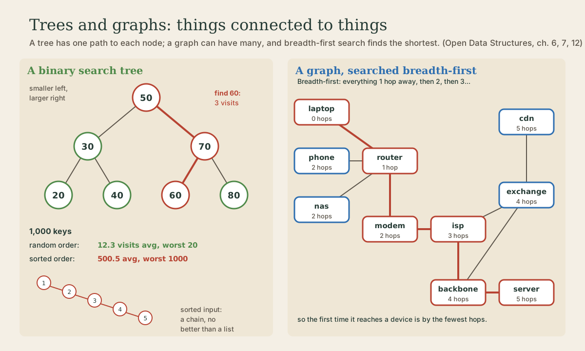
In a binary tree each node has at most two children, a left and a right ¹. A binary search tree adds a rule: for every node, all the keys in its left subtree are smaller than its own, and all the keys in its right subtree are larger ¹. To find a key, start at the root and compare: smaller, go left; larger, go right; equal, found. A search follows a single path down, never the whole tree ¹.

This program builds one, then measures how many nodes searches visit when 1,000 keys go in shuffled and when they go in already sorted. Save it as bst.py:

# bst.py: a binary search tree, and what insertion order does to its shape.
import random

class Node:
    def __init__(self, key):
        self.key = key
        self.left = None                # smaller keys go down here
        self.right = None               # larger keys go down here

def insert(root, key):
    """Add key to the tree and return its root."""
    if root is None:
        return Node(key)
    node = root
    while True:                         # walk down until there's an empty spot
        side = "left" if key < node.key else "right"
        child = getattr(node, side)
        if child is None:
            setattr(node, side, Node(key))
            return root
        node = child

def visits_to_find(root, key):
    """Count the nodes a search looks at before it reaches key."""
    node, visits = root, 1
    while node.key != key:
        node = node.left if key < node.key else node.right
        visits += 1
    return visits

def in_order(node):
    """Left subtree, this node, right subtree: the keys come out sorted."""
    if node is None:
        return []
    return in_order(node.left) + [node.key] + in_order(node.right)

small = None
for k in [50, 30, 70, 20, 40, 60, 80]:
    small = insert(small, k)
print("in order:", in_order(small))
print("visits to find 60:", visits_to_find(small, 60))

n = 1000
keys = list(range(n))
shuffled = keys[:]
random.seed(1)
random.shuffle(shuffled)
for name, order in [("random order", shuffled), ("sorted order", keys)]:
    root = None
    for k in order:
        root = insert(root, k)
    visits = [visits_to_find(root, k) for k in keys]
    print(f"{n} keys, {name:<13} average {sum(visits) / n:6.1f} visits, worst {max(visits)}")

getattr(node, side) reads the attribute named by the string side, and setattr sets it, so one line handles both directions. random.seed(1) makes the shuffle the same every run.

me@linuxbox:~$ python3 bst.py
in order: [20, 30, 40, 50, 60, 70, 80]
visits to find 60: 3
1000 keys, random order  average   12.3 visits, worst 20
1000 keys, sorted order  average  500.5 visits, worst 1000

Three things to see:

• An in-order traversal, visiting each node after its left subtree and before its right ¹, lists the keys sorted, for free.
• With keys in random order, a search among 1,000 keys visited about 12 nodes. For a randomly built tree, search paths are at most about 2 ln n long ¹; 2 ln 1000 is 13.8.
• With keys in sorted order, every new key was larger than everything before it, so each went right, and the “tree” became a chain 1,000 nodes deep: no better than a linked list, O(n) per search ¹.

Real data often arrives sorted, so practical search trees balance themselves, rearranging nodes as keys are added so the height stays proportional to log n; red-black trees are one widely used kind ¹. A related design, the B-tree, gives each node many children, sized so that one node fits in one disk block, and is the main data structure in filesystems such as Linux’s ext4, in every major database, and in key-value stores ¹.

Graphs

A graph is the general form: a set of vertices and a set of edges connecting pairs of them. Edges can be directed, one way only, or undirected. A path follows edges from vertex to vertex, and a path that returns to where it started is a cycle ¹. A tree is just a graph with no cycles ¹.

Graphs model anything defined by pairwise connections ¹: computers and network links, intersections and streets, or courses that share a student and so can’t have exams at the same time. Two more you’ve seen: git’s history, where a merge commit has two parents, so the history is a graph rather than a list; and package dependencies, which apt follows to install everything a program needs (Linux course).

Storing a graph

There are two standard ways ¹:

• An adjacency matrix: an n × n table with a 1 where there’s an edge. Checking whether two vertices are connected is O(1), but the table takes n² space even when most entries are 0.
• Adjacency lists: for each vertex, a list of its neighbors. Space is proportional to the number of vertices plus edges, and listing a vertex’s neighbors is direct.

Most real graphs are sparse, each vertex linked to only a few others, so adjacency lists are the usual choice. In Python, a dictionary of lists does it.

Breadth-first search

Breadth-first search (BFS) explores outward from a starting vertex: first its neighbors, then their neighbors, and so on. It keeps a queue of vertices to visit and a record of which ones it has already seen, so nothing is visited twice ¹. Because it finishes everything one hop away before anything two hops away, the first time it reaches a vertex is by a shortest path, counted in edges; remembering which vertex led to each one lets you read that path back ¹. It takes time proportional to the vertices plus the edges ¹.

This program runs BFS over a small made-up network, stored as adjacency lists. Save it as bfs.py:

# bfs.py: breadth-first search on a small made-up network, for fewest hops.
from collections import deque

links = {                               # adjacency lists: each device's neighbors
    "laptop":   ["router"],
    "phone":    ["router"],
    "router":   ["laptop", "phone", "nas", "modem"],
    "nas":      ["router"],
    "modem":    ["router", "isp"],
    "isp":      ["modem", "exchange", "backbone"],
    "exchange": ["isp", "backbone", "cdn"],
    "backbone": ["isp", "exchange", "server"],
    "cdn":      ["exchange"],
    "server":   ["backbone"],
}

def bfs(graph, start):
    """Visit nodes nearest-first; return each one's hop count and the node before it."""
    hops = {start: 0}
    came_from = {start: None}
    queue = deque([start])
    while queue:
        node = queue.popleft()          # first in, first out
        for neighbor in graph[node]:
            if neighbor not in hops:    # not seen yet
                hops[neighbor] = hops[node] + 1
                came_from[neighbor] = node
                queue.append(neighbor)
    return hops, came_from

def path(came_from, end):
    steps = []
    while end is not None:
        steps.append(end)
        end = came_from[end]
    return " -> ".join(reversed(steps))

hops, came_from = bfs(links, "laptop")
print("hops from laptop, in the order found:")
for node, h in hops.items():
    print(f"  {node:<9} {h}")
print(path(came_from, "server"))
print(path(came_from, "cdn"))

me@linuxbox:~$ python3 bfs.py
hops from laptop, in the order found:
  laptop    0
  router    1
  phone     2
  nas       2
  modem     2
  isp       3
  exchange  4
  backbone  4
  cdn       5
  server    5
laptop -> router -> modem -> isp -> backbone -> server
laptop -> router -> modem -> isp -> exchange -> cdn

All three structures of this module are working together: a deque as the queue, since it removes from the front in O(1) ³; a dict as the record of what’s been seen, with O(1) lookups; and lists of neighbors. Since a dict keeps the order its keys were added ⁴, hops lists the devices in the order BFS found them, nearest first.

Depth-first search

Depth-first search (DFS) does the opposite: it follows one path as far as it can, then backs up to the last branch it hasn’t explored. It’s breadth-first search with a stack instead of a queue, and is most naturally written as a recursive function ¹. DFS doesn’t find shortest paths, but it visits everything reachable just as well, and the order it works in makes it the tool for detecting cycles ¹.

Your turn

So

Trees connect nodes without loops, with one path from the root to each; the filesystem, the process tree, and git’s snapshots are trees. Binary search trees keep smaller keys left and larger right, so a search follows one path: about 12 visits among 1,000 random keys, but 500 on average when sorted input turns the tree into a chain, which is why practical trees balance themselves, and filesystems and databases use B-trees. Graphs are vertices and edges in general, usually stored as adjacency lists. Breadth-first search uses a queue to explore nearest-first and finds the fewest hops; depth-first search uses a stack to go deep first.